Univariate Bayesian spatial linear model

Fits a Bayesian spatial linear model with spatial process parameters and the noise-to-spatial variance ratio fixed to a value supplied by the user. The output contains posterior samples of the fixed effects, variance parameter, spatial random effects and, if required, leave-one-out predictive densities.

Usage

spLMexact(
  formula,
  data = parent.frame(),
  coords,
  cor.fn,
  priors,
  spParams,
  noise_sp_ratio,
  n.samples,
  loopd = FALSE,
  loopd.method = "exact",
  verbose = TRUE,
  ...
)

Arguments

formula: a symbolic description of the regression model to be fit. See example below.
data: an optional data frame containing the variables in the model. If not found in data, the variables are taken from environment(formula), typically the environment from which spLMexact is called.
coords: an $n \times 2$ matrix of the observation coordinates in $\mathbb{R}^2$ (e.g., easting and northing).
cor.fn: a quoted keyword that specifies the correlation function used to model the spatial dependence structure among the observations. Supported covariance model key words are: 'exponential' and 'matern'. See below for details.
priors: a list with each tag corresponding to a parameter name and containing prior details.
spParams: fixed value of spatial process parameters.
noise_sp_ratio: noise-to-spatial variance ratio.
n.samples: number of posterior samples to be generated.
loopd: logical. If loopd=TRUE, returns leave-one-out predictive densities, using method as given by loopd.method. Default is FALSE.
loopd.method: character. Ignored if loopd=FALSE. If loopd=TRUE, valid inputs are 'exact' and 'PSIS'. The option 'exact' corresponds to exact leave-one-out predictive densities which requires computation almost equivalent to fitting the model $n$ times. The option 'PSIS' is faster and finds approximate leave-one-out predictive densities using Pareto-smoothed importance sampling (Gelman et al. 2024).
verbose: logical. If verbose = TRUE, prints model description.
...: currently no additional argument.

Value

An object of class spLMexact, which is a list with the following tags -

samples: a list of length 3, containing posterior samples of fixed effects (beta), variance parameter (sigmaSq), spatial effects (z).
loopd: If loopd=TRUE, contains leave-one-out predictive densities.
model.params: Values of the fixed parameters that includes phi (spatial decay), nu (spatial smoothness) and noise_sp_ratio (noise-to-spatial variance ratio).

The return object might include additional data used for subsequent prediction and/or model fit evaluation.

Details

Suppose $\chi = (s_1, \ldots, s_n)$ denotes the $n$ spatial locations the response $y$ is observed. With this function, we fit a conjugate Bayesian hierarchical spatial model $$ \begin{aligned} y \mid z, \beta, \sigma^2 &\sim N(X\beta + z, \delta^2 \sigma^2 I_n), \quad z \mid \sigma^2 \sim N(0, \sigma^2 R(\chi; \phi, \nu)), \\ \beta \mid \sigma^2 &\sim N(\mu_\beta, \sigma^2 V_\beta), \quad \sigma^2 \sim \mathrm{IG}(a_\sigma, b_\sigma) \end{aligned} $$ where we fix the spatial process parameters $\phi$ and $\nu$, the noise-to-spatial variance ratio $\delta^2$ and the hyperparameters $\mu_\beta$, $V_\beta$, $a_\sigma$ and $b_\sigma$. We utilize a composition sampling strategy to sample the model parameters from their joint posterior distribution which can be written as $$ p(\sigma^2, \beta, z \mid y) = p(\sigma^2 \mid y) \times p(\beta \mid \sigma^2, y) \times p(z \mid \beta, \sigma^2, y). $$ We proceed by first sampling $\sigma^2$ from its marginal posterior, then given the samples of $\sigma^2$, we sample $\beta$ and subsequently, we sample $z$ conditioned on the posterior samples of $\beta$ and $\sigma^2$ (Banerjee 2020).

References

Banerjee S (2020). "Modeling massive spatial datasets using a conjugate Bayesian linear modeling framework." Spatial Statistics, 37, 100417. ISSN 2211-6753. doi:10.1016/j.spasta.2020.100417 .

Vehtari A, Simpson D, Gelman A, Yao Y, Gabry J (2024). "Pareto Smoothed Importance Sampling." Journal of Machine Learning Research, 25(72), 1-58. URL https://jmlr.org/papers/v25/19-556.html.

Author

Soumyakanti Pan span18@ucla.edu,
Sudipto Banerjee sudipto@ucla.edu

Examples

# load data
data(simGaussian)
dat <- simGaussian[1:100, ]

# setup prior list
muBeta <- c(0, 0)
VBeta <- cbind(c(1.0, 0.0), c(0.0, 1.0))
sigmaSqIGa <- 2
sigmaSqIGb <- 0.1
prior_list <- list(beta.norm = list(muBeta, VBeta),
                   sigma.sq.ig = c(sigmaSqIGa, sigmaSqIGb))

# supply fixed values of model parameters
phi0 <- 3
nu0 <- 0.75
noise.sp.ratio <- 0.8

mod1 <- spLMexact(y ~ x1, data = dat,
                  coords = as.matrix(dat[, c("s1", "s2")]),
                  cor.fn = "matern",
                  priors = prior_list,
                  spParams = list(phi = phi0, nu = nu0),
                  noise_sp_ratio = noise.sp.ratio,
                  n.samples = 100,
                  loopd = TRUE, loopd.method = "exact")
#> ----------------------------------------
#> 	Model description
#> ----------------------------------------
#> Model fit with 100 observations.
#> 
#> Number of covariates 2 (including intercept).
#> 
#> Using the matern spatial correlation function.
#> 
#> Priors:
#> 	beta: Gaussian
#> 	mu:	0.00	0.00	
#> 	cov:
#> 	1.00	0.00	
#> 	0.00	1.00	
#> 
#> 	sigma.sq: Inverse-Gamma
#> 	shape = 2.00, scale = 0.10.
#> 
#> Spatial process parameters:
#> 	phi = 3.00, and, nu = 0.75.
#> Noise-to-spatial variance ratio = 0.80.
#> 
#> Number of posterior samples = 100.
#> 
#> LOO-PD calculation method = exact.
#> ----------------------------------------

beta.post <- mod1$samples$beta
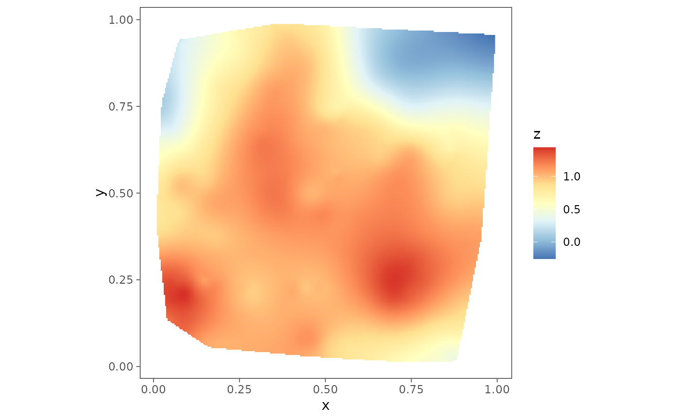
z.post.median <- apply(mod1$samples$z, 1, median)
dat$z.post.median <- z.post.median
plot1 <- surfaceplot(dat, coords_name = c("s1", "s2"),
                     var_name = "z_true")
plot2 <- surfaceplot(dat, coords_name = c("s1", "s2"),
                     var_name = "z.post.median")
plot1

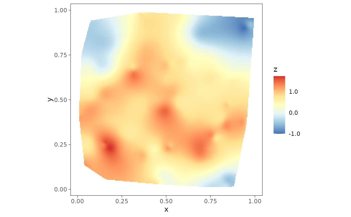plot2