spStack: Bayesian Geostatistics Using Predictive Stacking • spStack

Introduction

Geostatistics refers to the study of a spatially distributed variable of interest, which in theory is defined at every point over a bounded study region of interest. Statistical modelling and analysis for spatially oriented point-referenced outcomes play a crucial role in diverse scientific applications such as earth and environmental sciences, ecology, epidemiology, and economics. With the advent of Markov chain Monte Carlo (MCMC) algorithms, Bayesian hierarchical models have gained massive popularity in analyzing such point-referenced or, geostatistical data. These models involve latent spatial processes characterized by spatial process parameters, which besides lacking substantive relevance in scientific contexts, are also weakly identified and hence, impedes convergence of MCMC algorithms. Thus, even for moderately large datasets (~ $10^3$ or higher), the computation for MCMC becomes too onerous for practical use.

We introduce the R package spStack that implements Bayesian inference for a class of geostatistical models, where we obviate the issues mentioned by sampling from analytically available posterior distributions conditional upon some candidate values of the spatial process parameters and, subsequently assimilate inference from these individual posterior distributions using Bayesian predictive stacking. Besides delivering competitive predictive performance as compared to fully Bayesian inference using MCMC, our proposed algorithm is embarrassingly parallel, thus drastically improves runtime and elevating the utility of the package for a diverse group of practitioners with limited computational resources at their disposal. This package, to the best of our knowledge, is the first to implement stacking for Bayesian analysis of spatial data.

Technical details surrounding the methodology can be found in the articles Zhang, Tang, and Banerjee (2024) which discuss the case where the distribution of the point-referenced outcomes are Gaussian, and, in Pan et al. (2024) where the case of non-Gaussian outcomes is explored. The code for this package is written primarily in C/C++ with additional calls to FORTRAN routines for optimized linear algebra operations. We leverage the F77_NAME macro to interface with legacy FORTRAN functions in conjunction with efficient matrix computation libraries such as BLAS (Basic Linear Algebra Subprograms) and LAPACK (Linear Algebra Package) to implement our stacking algorithm.

The remainder of the vignette evolves as follows - the next two sections discuss Bayesian hierarchical spatial models for Gaussian and non-Gaussian outcomes, which is followed by a section providing brief details on predictive stacking and a section dedicated for illustration of functions in the package.

Bayesian Gaussian spatial regression models

Let $\chi = \{s_1, \ldots, s_n\} \in \mathcal{D}$ be a be a set of $n$ spatial locations yielding measurements $y = (y_1, \ldots, y_n)^{ \scriptstyle \top }$ with known values of predictors at these locations collected in the $n \times p$ full rank matrix $X = [x(s_1), \ldots, x(s_n)]^{ \scriptstyle \top }$ . A customary geostatistical model is $\begin{equation} y_i = x(s_i)^{ \scriptstyle \top }\beta + z(s_i) + \epsilon_i, \quad i = 1, \ldots, n, \end{equation}$ where $\beta$ is the $p \times 1$ vector of slopes, $z(s) \sim \mathrm{GP}(0, R(\cdot, \cdot; {\theta_{\text{sp}}}))$ is a zero-centered spatial Gaussian process on $\mathcal{D}$ with spatial correlation function $R(\cdot, \cdot; {\theta_{\text{sp}}})$ characterized by process parameters ${\theta_{\text{sp}}}$ , $\sigma^2$ is the spatial variance parameter (“partial sill”) and $\epsilon_i \sim \mathcal{N}(0, \tau^2), i = 1, \ldots, n$ are i.i.d. with variance $\tau^2$ (“nugget”) capturing measurement error. The spatial process $z(\cdot)$ is assumed to be independent of the measurement errors $\{\epsilon_i, i = 1, \ldots, n\}$ . Let $z = (z(s_1), \ldots, z(s_n))^{ \scriptstyle \top }$ denotes the realization of the spatial process on $\chi$ and $n \times n$ correlation matrix $R(\chi; {\theta_{\text{sp}}}) = (R(s_i, s_j {\theta_{\text{sp}}}))_{1 \leq i,j \leq n}$ . We build a conjugate Bayesian hierarchical spatial model, $\begin{equation} \begin{split} y \mid z, \beta, \sigma^2 &\sim N(X\beta + z, \delta^2 \sigma^2 I_n), \\ z \mid \sigma^2 &\sim N(0, \sigma^2 R(\chi; {\theta_{\text{sp}}})), \\ \beta \mid \sigma^2 &\sim N(\mu_\beta, \sigma^2 V_\beta), \quad \sigma^2 \sim \mathrm{IG}(a_\sigma, b_\sigma), \end{split} \end{equation}$ where we fix the noise-to-spatial variance ratio $\delta^2 = \tau^2 / \sigma^2$ , the process parameters ${\theta_{\text{sp}}}$ and the hyperparameters $\mu_\beta$ , $V_\beta$ , $a_\sigma$ and $b_\sigma$ . In this package, we use the Matern covariogram specified by spatial decay parameter $\phi$ and smoothness parameter $\nu$ i.e., ${\theta_{\text{sp}}}= \{\phi, \nu\}$ , given by $\begin{equation} R(s, s'; {\theta_{\text{sp}}}) = \frac{(\phi \lvert s - s' \rvert)^\nu}{2^{\nu - 1} \Gamma(\nu)} K_\nu (\phi \lvert s - s' \rvert)). \end{equation}$ We utilize a composition sampling strategy to sample the model parameters from their joint posterior distribution which can be written as $\begin{equation} p(\sigma^2, \beta, z \mid y) = p(\sigma^2 \mid y) \times p(\beta \mid \sigma^2, y) \times p(z \mid \beta, \sigma^2, y). \end{equation}$ We proceed by first sampling $\sigma^2$ from its marginal posterior, then given the samples of $\sigma^2$ , we sample $\beta$ and subsequently, we sample $z$ conditioned on the posterior samples of $\beta$ and $\sigma^2$ (Banerjee 2020). The function spLMexact() delivers samples from this posterior distribution. More details can be found in Zhang, Tang, and Banerjee (2024).

Bayesian non-Gaussian spatial regression models

Analyzing non-Gaussian spatial data typically requires introducing spatial dependence in generalized linear models through the link function of an exponential family distribution. Let $y(s)$ be the outcome at location $s \in \mathcal{D}$ endowed with a probability law from the natural exponential family, which we denote by $\begin{equation} y(s) \sim \mathrm{EF}(x(s)^{ \scriptstyle \top }\beta + z(s); b, \psi_y) \end{equation}$ for some positive parameter $b > 0$ and unit log partition function $\psi_y$ . Fixed effects regression and spatial dependence, e.g., $x(s)^{{ \scriptstyle \top }}\beta + z(s)$ , is introduced in the natural parameter, where $x(s)$ is a $p \times 1$ vector of predictors referenced with respect to $s$ , $\beta$ is a $p \times 1$ vector of slopes measuring the trend, $z(s)$ is a zero-centered spatial process on $\mathcal{D}$ specified by a scale parameter $\sigma_z$ and a spatial correlation function $R(\cdot, \cdot ; {\theta_{\text{sp}}})$ with ${\theta_{\text{sp}}}$ consisting of spatial-temporal decay and smoothness parameters.

Unlike in Gaussian likelihoods, inference is considerably encumbered by the inability to analytically integrate out the random effects and reduce the dimension of the parameter space. Iterative algorithms such as Markov Chain Monte Carlo (MCMC), thus attempt to sample from a very high-dimensional posterior distribution, and convergence is often hampered by high auto-correlations and weakly identified spatial process parameters ${\theta_{\text{sp}}}$ .

We consider the following three cases -

Point-referenced Poisson count data: Here $b = 1$ and $\psi_y(t) = e^t$ . $\begin{equation} \begin{split} y(s_i) &\sim \mathrm{Poisson}(\lambda(s_i)), \quad i = 1, \dots, n.\\ \lambda(s_i) & = \exp(x(s_i)^{ \scriptstyle \top }\beta + z(s_i)) \end{split} \end{equation}$
Point-referenced binomial count data: Here $b = m(s_i)$ for each $i$ and $\psi_y(t) = \log(1 + e^t)$ . $\begin{equation} \begin{split} y(s_i) &\sim \mathrm{Binomial}(m(s_i), \pi(s_i)), \quad i = 1, \dots, n.\\ \pi(s_i) & = \mathrm{ilogit}(x(s_i)^{ \scriptstyle \top }\beta + z(s_i)) \end{split} \end{equation}$
Point-referenced binary data: Here $b = 1$ and $\psi_y(t) = \log(1 + e^t)$ . $\begin{equation} \begin{split} y(s_i) &\sim \mathrm{Bernoulli}(\pi(s_i)), \quad i = 1, \dots, n.\\ \pi(s_i) & = \mathrm{ilogit}(x(s_i)^{ \scriptstyle \top }\beta + z(s_i)) \end{split} \end{equation}$

Following Bradley and Clinch (2024), we introduce a Bayesian hierarchical spatial model as $\begin{equation} \begin{split} y(s_i) \mid \beta, z, \xi & \sim \mathrm{EF}\left(x(s_i)^{ \scriptstyle \top }\beta + z(s_i) + \xi_i - \mu_i; b_i, \psi_y\right), i = 1, \ldots, n\\ \beta \mid \sigma^2_\beta &\sim N(0, \sigma^2_\beta V_\beta), \quad \sigma^2_\beta \sim \mathrm{IG}(\nu_\beta/2, \nu_\beta/2)\\ z \mid \sigma^2_z &\sim N\left(0, \sigma^2_z R(\chi; {\theta_{\text{sp}}})\right), \quad \sigma^2_z \sim \mathrm{IG}(\nu_z/2, \nu_z/2),\\ \xi \mid \beta, z, \sigma^2_\xi, \alpha_\epsilon &\sim \mathrm{GCM_c}\left(\tilde{\mu}_\xi, H_\xi, \epsilon, \kappa_\xi; \psi_\xi\right), \end{split} \end{equation}$ where $\mu = (\mu_1, \ldots, \mu_n)^{ \scriptstyle \top }$ denotes the discrepancy parameter. We fix the spatial process parameters ${\theta_{\text{sp}}}$ , the boundary adjustment parameter $\epsilon$ and the hyperparameters $V_\beta$ , $\nu_\beta$ , $\nu_z$ and $\sigma^2_\xi$ . The term $\xi$ is known as the fine-scale variation term which is given a conditional generalized conjugate multivariate distribution ( $\mathrm{GCM_c}$ ) as prior. For details, see Pan et al. (2024).

Predictive stacking

Following Yao et al. (2018), we consider a set of candidate models based on a grid of values of the parameters in $\{ {\theta_{\text{sp}}}, \delta^2 \}$ for the Gaussian case, and $\{ {\theta_{\text{sp}}}, \epsilon \}$ for the non-Gaussian case, as will be supplied by the user. We build a set of candidate models based on the Cartesian product of the collection of values for each individual parameter as $\mathcal{M} = \{M_1, \ldots, M_G\}$ . Then, for each $g = 1, \ldots, G$ , we sample from the posterior distribution $p(\sigma^2, \beta, z \mid y, M_g)$ under the model $M_g$ and find leave-one-out predictive densities $p(y_i \mid y_{-i}, M_g)$ . Then we solve the optimization problem $\begin{equation} \begin{split} \max_{w_1, \ldots, w_G}& \, \frac{1}{n} \sum_{i = 1}^n \log \sum_{g = 1}^G w_g p(y_i \mid y_{-i}, M_g) \\ \text{subject to} & \quad w_g \geq 0, \sum_{g = 1}^G w_g = 1 \end{split} \end{equation}$ to find the optimal stacking weights $\hat{w}_1, \ldots, \hat{w}_G$ . After obtaining the optimal stacking weights, posterior inference of any quantity of interest subsequently proceed from the stacked posterior, $\begin{equation} \tilde{p}(\cdot \mid y) = \sum_{g = 1}^G \hat{w}_g p(\cdot \mid y, M_g). \end{equation}$

Illustrations

In this section, we thoroughly illustrate our method on synthetic Gaussian as well as non-Gaussian spatial data and provide code to analyze the output of our functions. We start by loading the package.

library(spStack)

Some synthetic spatial data are lazy-loaded which includes synthetic spatial Gaussian data simGaussian, Poisson data simPoisson, binomial data simBinom and binary data simBinary. One can use the function sim_spData() to simulate spatial data. We will be applying our functions on these datasets.

Analysis of spatial Gaussian data

We first load the data simGaussian and set up the priors. Supplying the priors is optional. See the documentation of spLMexact() to learn more about the default priors. Besides, setting the priors, we also fix the values of the spatial process parameters and the noise-to-spatial variance ratio.

data("simGaussian")
dat <- simGaussian[1:200, ] # work with first 200 rows

muBeta <- c(0, 0)
VBeta <- cbind(c(10.0, 0.0), c(0.0, 10.0))
sigmaSqIGa <- 2
sigmaSqIGb <- 2
phi0 <- 2
nu0 <- 0.5
noise_sp_ratio <- 0.8
prior_list <- list(beta.norm = list(muBeta, VBeta),
                   sigma.sq.ig = c(sigmaSqIGa, sigmaSqIGb))
nSamples <- 2000

We then pass these parameters into the main function.

set.seed(1729)
mod1 <- spLMexact(y ~ x1, data = dat,
                  coords = as.matrix(dat[, c("s1", "s2")]),
                  cor.fn = "matern",
                  priors = prior_list,
                  spParams = list(phi = phi0, nu = nu0),
                  noise_sp_ratio = noise_sp_ratio, n.samples = nSamples,
                  loopd = TRUE, loopd.method = "exact",
                  verbose = TRUE)
#> ----------------------------------------
#>  Model description
#> ----------------------------------------
#> Model fit with 200 observations.
#> 
#> Number of covariates 2 (including intercept).
#> 
#> Using the matern spatial correlation function.
#> 
#> Priors:
#>  beta: Gaussian
#>  mu: 0.00    0.00    
#>  cov:
#>  10.00   0.00    
#>  0.00    10.00   
#> 
#>  sigma.sq: Inverse-Gamma
#>  shape = 2.00, scale = 2.00.
#> 
#> Spatial process parameters:
#>  phi = 2.00, and, nu = 0.50.
#> Noise-to-spatial variance ratio = 0.80.
#> 
#> Number of posterior samples = 2000.
#> 
#> LOO-PD calculation method = exact.
#> ----------------------------------------

Next, we can summarize the posterior samples of the fixed effects as follows.

post_beta <- mod1$samples$beta
summary_beta <- t(apply(post_beta, 1, function(x) quantile(x, c(0.025, 0.5, 0.975))))
rownames(summary_beta) <- mod1$X.names
print(summary_beta)
#>                 2.5%      50%    97.5%
#> (Intercept) 1.388249 2.129140 2.932428
#> x1          4.865843 4.954446 5.045627

If interested in finding leave-one-out predictive densities (LOO-PD) for this model, set loopd to TRUE and provide a loopd.method. Valid inputs for loopd.method are "exact" and "PSIS" which finds exact LOO-PD using closed form expressions and approximate LOO-PD using Pareto smoothed importance sampling (Vehtari, Gelman, and Gabry 2017).

mod2 <- spLMexact(y ~ x1, data = dat,
                  coords = as.matrix(dat[, c("s1", "s2")]),
                  cor.fn = "matern",
                  priors = prior_list,
                  spParams = list(phi = phi0, nu = nu0),
                  noise_sp_ratio = noise_sp_ratio, n.samples = nSamples,
                  loopd = TRUE, loopd.method = "PSIS",
                  verbose = FALSE)

Out of curiosity, we compare the LOO-PD obtained by the two methods.

loopd_exact <- mod1$loopd
loopd_psis <- mod2$loopd
loopd_df <- data.frame(exact = loopd_exact, psis = loopd_psis)

library(ggplot2)
plot1 <- ggplot(data = loopd_df, aes(x = exact)) +
  geom_point(aes(y = psis), size = 1, alpha = 0.5) +
  geom_abline(slope = 1, intercept = 0, color = "red", alpha = 0.5) +
  xlab("Exact") + ylab("PSIS") + theme_bw() +
  theme(panel.background = element_blank(), aspect.ratio = 1)
plot1

Next, we move on to the Bayesian spatial stacking algorithm for Gaussian data. We supply the same prior list and provide some candidate values of spatial process parameters and noise-to-spatial variance ratio.

mod3 <- spLMstack(y ~ x1, data = dat,
                  coords = as.matrix(dat[, c("s1", "s2")]),
                  cor.fn = "matern",
                  priors = prior_list,
                  params.list = list(phi = c(1.5, 3, 5),
                                     nu = c(0.5, 1, 1.5),
                                     noise_sp_ratio = c(0.5, 1.5)),
                  n.samples = 1000, loopd.method = "exact",
                  parallel = FALSE, solver = "ECOS", verbose = TRUE)
#> 
#> STACKING WEIGHTS:
#> 
#>            | phi | nu  | noise_sp_ratio | weight |
#> +----------+-----+-----+----------------+--------+
#> | Model 1  |  1.5|  0.5|             0.5| 0.000  |
#> | Model 2  |  3.0|  0.5|             0.5| 0.000  |
#> | Model 3  |  5.0|  0.5|             0.5| 0.000  |
#> | Model 4  |  1.5|  1.0|             0.5| 0.226  |
#> | Model 5  |  3.0|  1.0|             0.5| 0.000  |
#> | Model 6  |  5.0|  1.0|             0.5| 0.774  |
#> | Model 7  |  1.5|  1.5|             0.5| 0.000  |
#> | Model 8  |  3.0|  1.5|             0.5| 0.000  |
#> | Model 9  |  5.0|  1.5|             0.5| 0.000  |
#> | Model 10 |  1.5|  0.5|             1.5| 0.000  |
#> | Model 11 |  3.0|  0.5|             1.5| 0.000  |
#> | Model 12 |  5.0|  0.5|             1.5| 0.000  |
#> | Model 13 |  1.5|  1.0|             1.5| 0.000  |
#> | Model 14 |  3.0|  1.0|             1.5| 0.000  |
#> | Model 15 |  5.0|  1.0|             1.5| 0.000  |
#> | Model 16 |  1.5|  1.5|             1.5| 0.000  |
#> | Model 17 |  3.0|  1.5|             1.5| 0.000  |
#> | Model 18 |  5.0|  1.5|             1.5| 0.000  |
#> +----------+-----+-----+----------------+--------+

The user can check the solver status and runtime by issuing the following.

print(mod3$solver.status)
#> [1] "optimal"
print(mod3$run.time)
#>    user  system elapsed 
#>   2.627   2.969   1.683

To sample from the stacked posterior, the package provides a helper function called stackedSampler(). Subsequent inference proceeds from these samples obtained from the stacked posterior.

post_samps <- stackedSampler(mod3)

We then collect the samples of the fixed effects and summarize them as follows.

post_beta <- post_samps$beta
summary_beta <- t(apply(post_beta, 1, function(x) quantile(x, c(0.025, 0.5, 0.975))))
rownames(summary_beta) <- mod3$X.names
print(summary_beta)
#>                  2.5%      50%    97.5%
#> (Intercept) 0.9303819 2.185930 2.949784
#> x1          4.8678581 4.954272 5.030520

Here, we compare the posterior samples of the spatial random effects with their corresponding true values.

post_z <- post_samps$z
post_z_summ <- t(apply(post_z, 1, function(x) quantile(x, c(0.025, 0.5, 0.975))))
z_combn <- data.frame(z = dat$z_true, zL = post_z_summ[, 1],
                      zM = post_z_summ[, 2], zU = post_z_summ[, 3])

plotz <- ggplot(data = z_combn, aes(x = z)) +
  geom_point(aes(y = zM), size = 0.75, color = "darkblue", alpha = 0.5) +
  geom_errorbar(aes(ymin = zL, ymax = zU), width = 0.05, alpha = 0.15, 
                color = "skyblue") + 
  geom_abline(slope = 1, intercept = 0, color = "red") +
  xlab("True z") + ylab("Stacked posterior of z") + theme_bw() +
  theme(panel.background = element_blank(), aspect.ratio = 1)
plotz

The package also provides functions to plot interpolated spatial surfaces in order for visualization purposes. The function surfaceplot() creates a single spatial surface plot, while surfaceplot2() creates two side-by-side surface plots. We are using the later to visually inspect the interpolated spatial surfaces of the true spatial effects and their posterior medians.

postmedian_z <- apply(post_z, 1, median)
dat$z_hat <- postmedian_z
plot_z <- surfaceplot2(dat, coords_name = c("s1", "s2"),
                       var1_name = "z_true", var2_name = "z_hat")
library(ggpubr)
ggarrange(plotlist = plot_z, common.legend = TRUE, legend = "right")

Analysis of spatial non-Gaussian data

In this package, we offer functions for Bayesian analysis Poisson and binomial count data as well as binary data.

Spatial Poisson count data

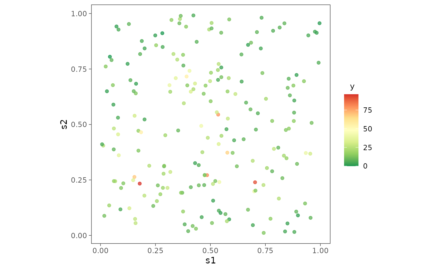
We first load and plot the point-referenced Poisson count data.

data("simPoisson")
dat <- simPoisson[1:200, ] # work with first 200 observations

ggplot(dat, aes(x = s1, y = s2)) +
  geom_point(aes(color = y), alpha = 0.75) +
  scale_color_distiller(palette = "RdYlGn", direction = -1, 
                        label = function(x) sprintf("%.0f", x)) +
  guides(alpha = 'none') + theme_bw() +
  theme(axis.ticks = element_line(linewidth = 0.25),
        panel.background = element_blank(), panel.grid = element_blank(),
        legend.title = element_text(size = 10, hjust = 0.25),
        legend.box.just = "center", aspect.ratio = 1)

Next, we demonstrate the function spGLMexact() which delivers posterior samples of the fixed effects and the spatial random effects. The option family must be specified correctly while using this function. For instance, in this example family = "poisson". We provide fixed values of the spatial process parameters and the boundary adjustment parameter, given by the argument boundary, which if not supplied, defaults to 0.5. For details on the priors and its default value, see function documentation.

mod1 <- spGLMexact(y ~ x1, data = dat, family = "poisson",
                   coords = as.matrix(dat[, c("s1", "s2")]), cor.fn = "matern",
                   spParams = list(phi = phi0, nu = nu0),
                   boundary = 0.5,
                   n.samples = 1000, verbose = TRUE)
#> ----------------------------------------
#>  Model description
#> ----------------------------------------
#> Model fit with 200 observations.
#> 
#> Family = poisson.
#> 
#> Number of covariates 2 (including intercept).
#> 
#> Using the matern spatial correlation function.
#> 
#> Priors:
#>  beta: Gaussian
#>  mu: 0.00    0.00    
#>  cov:
#>  100.00  0.00    
#>  0.00    100.00  
#> 
#>  sigmaSq.beta ~ IG(nu.beta/2, nu.beta/2)
#>  sigmaSq.z ~ IG(nu.z/2, nu.z/2)
#>  nu.beta = 2.10, nu.z = 2.10.
#>  sigmaSq.xi = 0.10.
#>  Boundary adjustment parameter = 0.50.
#> 
#> Spatial process parameters:
#>  phi = 2.00, and, nu = 0.50.
#> 
#> Number of posterior samples = 1000.
#> ----------------------------------------

We next collect the samples of the fixed effects and summarize them. The true value of the fixed effects with which the data was simulated is $\beta = (2, -0.5)$ (for more details, see the documentation of the data simPoisson).

post_beta <- mod1$samples$beta
summary_beta <- t(apply(post_beta, 1, function(x) quantile(x, c(0.025, 0.5, 0.975))))
rownames(summary_beta) <- mod1$X.names
print(summary_beta)
#>                   2.5%        50%      97.5%
#> (Intercept) -0.1302807  1.9026041  4.3045317
#> x1          -0.6664152 -0.5545303 -0.4543145

Next, we move on to the function spGLMstack() that will implement our proposed stacking algorithm. The argument loopd.controls is used to provide details on what algorithm to be used to find LOO-PD. Valid options for the tag method is "exact" and "CV". We use $K$ -fold cross-validation by assigning method = "CV"and CV.K = 10. The tag nMC decides the number of Monte Carlo samples to be used to find the LOO-PD.

mod2 <- spGLMstack(y ~ x1, data = dat, family = "poisson",
                   coords = as.matrix(dat[, c("s1", "s2")]), cor.fn = "matern",
                   params.list = list(phi = c(3, 7, 10), nu = c(0.5, 1.5),
                                      boundary = c(0.5, 0.6)),
                   n.samples = 1000,
                   loopd.controls = list(method = "CV", CV.K = 10, nMC = 1000),
                   parallel = TRUE, solver = "ECOS", verbose = TRUE)
#> 
#> STACKING WEIGHTS:
#> 
#>            | phi | nu  | boundary | weight |
#> +----------+-----+-----+----------+--------+
#> | Model 1  |    3|  0.5|       0.5| 0.000  |
#> | Model 2  |    7|  0.5|       0.5| 0.000  |
#> | Model 3  |   10|  0.5|       0.5| 0.000  |
#> | Model 4  |    3|  1.5|       0.5| 0.000  |
#> | Model 5  |    7|  1.5|       0.5| 0.000  |
#> | Model 6  |   10|  1.5|       0.5| 0.000  |
#> | Model 7  |    3|  0.5|       0.6| 0.000  |
#> | Model 8  |    7|  0.5|       0.6| 0.000  |
#> | Model 9  |   10|  0.5|       0.6| 0.000  |
#> | Model 10 |    3|  1.5|       0.6| 0.175  |
#> | Model 11 |    7|  1.5|       0.6| 0.825  |
#> | Model 12 |   10|  1.5|       0.6| 0.000  |
#> +----------+-----+-----+----------+--------+

We can extract information on solver status and runtime by the following.

print(mod2$solver.status)
#> [1] "optimal"
print(mod2$run.time)
#>    user  system elapsed 
#>  25.262  34.958  15.279

We first obtain final posterior samples by sampling from the stacked sampler.

post_samps <- stackedSampler(mod2)

Subsequently, we summarize the posterior samples of the fixed effects.

post_beta <- post_samps$beta
summary_beta <- t(apply(post_beta, 1, function(x) quantile(x, c(0.025, 0.5, 0.975))))
rownames(summary_beta) <- mod3$X.names
print(summary_beta)
#>                   2.5%        50%      97.5%
#> (Intercept) -0.8032363  2.0460414  3.8253354
#> x1          -0.6275769 -0.5471968 -0.4529202

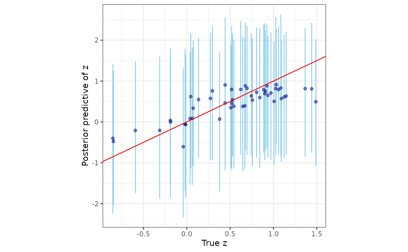
Finally, we analyze the posterior samples of the spatial random effects.

post_z <- post_samps$z
post_z_summ <- t(apply(post_z, 1, function(x) quantile(x, c(0.025, 0.5, 0.975))))
z_combn <- data.frame(z = dat$z_true, zL = post_z_summ[, 1],
                      zM = post_z_summ[, 2], zU = post_z_summ[, 3])

plotz <- ggplot(data = z_combn, aes(x = z)) +
  geom_point(aes(y = zM), size = 0.75, color = "darkblue", alpha = 0.5) +
  geom_errorbar(aes(ymin = zL, ymax = zU), width = 0.05, alpha = 0.15,
                color = "skyblue") +
  geom_abline(slope = 1, intercept = 0, color = "red") +
  xlab("True z") + ylab("Stacked posterior of z") + theme_bw() +
  theme(panel.background = element_blank(), aspect.ratio = 1)
plotz

We can also compare the interpolated spatial surfaces of the true spatial effects with that of their posterior median.

postmedian_z <- apply(post_z, 1, median)
dat$z_hat <- postmedian_z
plot_z <- surfaceplot2(dat, coords_name = c("s1", "s2"),
                       var1_name = "z_true", var2_name = "z_hat")
library(ggpubr)
ggarrange(plotlist = plot_z, common.legend = TRUE, legend = "right")

Spatial binomial count data

Here, we present only the spGLMexact() function for brevity. The only argument that will change from that of in the case of spatial Poisson data is the structure of formula that defines the model.

data("simBinom")
dat <- simBinom[1:200, ] # work with first 200 rows

mod1 <- spGLMexact(cbind(y, n_trials) ~ x1, data = dat, family = "binomial",
                   coords = as.matrix(dat[, c("s1", "s2")]), cor.fn = "matern",
                   spParams = list(phi = 3, nu = 0.5),
                   boundary = 0.5, n.samples = 1000, verbose = FALSE)

Similarly, we collect the posterior samples of the fixed effects and summarize them. The true value of the fixed effects with which the data was simulated is $\beta = (0.5, -0.5)$ .

post_beta <- mod1$samples$beta
summary_beta <- t(apply(post_beta, 1, function(x) quantile(x, c(0.025, 0.5, 0.975))))
rownames(summary_beta) <- mod1$X.names
print(summary_beta)
#>                   2.5%        50%      97.5%
#> (Intercept) -1.2039026  0.7229478  2.5872269
#> x1          -0.5815266 -0.4016808 -0.2365151

Spatial binary data

Finally, we present only the spGLMexact() function for spatial binary data to avoid repetition. In this case, unlike the binomial model, almost nothing changes from that of in the case of spatial Poisson data.

data("simBinary")
dat <- simBinary[1:200, ]

mod1 <- spGLMexact(y ~ x1, data = dat, family = "binary",
                   coords = as.matrix(dat[, c("s1", "s2")]), cor.fn = "matern",
                   spParams = list(phi = 4, nu = 0.4),
                   boundary = 0.5, n.samples = 1000, verbose = FALSE)

Similarly, we collect the posterior samples of the fixed effects and summarize them. The true value of the fixed effects with which the data was simulated is $\beta = (0.5, -0.5)$ .

post_beta <- mod1$samples$beta
summary_beta <- t(apply(post_beta, 1, function(x) quantile(x, c(0.025, 0.5, 0.975))))
rownames(summary_beta) <- mod1$X.names
print(summary_beta)
#>                   2.5%        50%      97.5%
#> (Intercept) -1.1291296  0.3061828 1.70795510
#> x1          -0.6507851 -0.3088350 0.04471555

Conclusion

We have devised and demonstrated Bayesian predictive stacking to be an effective tool for estimating spatial regression models and yielding robust predictions for Gaussian as well as non-Gaussian spatial data. We develop and exploit analytically accessible distribution theory pertaining to Bayesian analysis of linear mixed model and generalized linear mixed models that enables us to directly sample from the posterior distributions. The focus of this package is on effectively combining inference across different closed-form posterior distributions by circumventing inference on weakly identified parameters. Future developments and investigations will consider zero-inflated non-Gaussian data and adapting to variants of Gaussian process models that scale inference to massive datasets by circumventing the Cholesky decomposition of dense covariance matrices.

References

Banerjee, Sudipto. 2020. “Modeling Massive Spatial Datasets Using a Conjugate Bayesian Linear Modeling Framework.” Spatial Statistics 37: 100417. https://doi.org/10.1016/j.spasta.2020.100417.

Bradley, Jonathan R., and Madelyn Clinch. 2024. “Generating Independent Replicates Directly from the Posterior Distribution for a Class of Spatial Hierarchical Models.” Journal of Computational and Graphical Statistics 0 (0): 1–17. https://doi.org/10.1080/10618600.2024.2365728.

Pan, Soumyakanti, Lu Zhang, Jonathan R. Bradley, and Sudipto Banerjee. 2024. “Bayesian Inference for Spatial-Temporal Non-Gaussian Data Using Predictive Stacking.” https://arxiv.org/abs/2406.04655.

Vehtari, Aki, Andrew Gelman, and Jonah Gabry. 2017. “Practical Bayesian Model Evaluation Using Leave-One-Out Cross-Validation and WAIC.” Statistics and Computing 27 (5): 1413–32. https://doi.org/10.1007/s11222-016-9696-4.

Yao, Yuling, Aki Vehtari, Daniel Simpson, and Andrew Gelman. 2018. “Using Stacking to Average Bayesian Predictive Distributions (with Discussion).” Bayesian Analysis 13 (3): 917–1007. https://doi.org/10.1214/17-BA1091.

Zhang, Lu, Wenpin Tang, and Sudipto Banerjee. 2024. “Bayesian Geostatistics Using Predictive Stacking.” https://arxiv.org/abs/2304.12414.