In this article, we discuss the function -
This function can be used to obtain posterior predictive inference at
unobserved locations in space or time. It is applied on the output of
functions spLMexact(), spLMstack(),
spGLMexact(), spGLMstack(),
stvcLMexact(), stvcLMstack(),
stvcGLMexact() and stvcGLMstack(). We use the
synthetic datasets simSpatial and
simSpaceTime: we fit the models on the first rows of a
dataset and predict at the next ones, where we compare the predictions
with the true values.
The joint argument in posteriorPredict()
indicates if the predictions at the new locations or times are to be
made based on the joint posterior predictive distribution or not. If
joint=FALSE, then the individual predictions are made from
their corresponding posterior predictive distributions.
Prediction in spatial linear model
Define the collection of candidate models and fit using
spLMstack() to the Gaussian response y_gauss
of simSpatial.
# training and test data sizes
n_train <- 200
n_pred <- 50

data("simSpatial")
dat_train <- simSpatial[1:n_train, ]
dat_pred <- simSpatial[n_train + 1:n_pred, ]

cand.mod <- candidateModels(list(phi = c(2, 4, 6, 8),
                                 nu = c(0.5, 1, 1.5, 1.75),
                                 noise_sp_ratio = c(0.1, 0.5)),
                            "cartesian")

mod1 <- spLMstack(y_gauss ~ x1 + x2, data = dat_train,
                  coords = as.matrix(dat_train[, c("s1", "s2")]),
                  cor.fn = "matern",
                  candidate.models = cand.mod,
                  n.samples = 1000, loopd.method = "exact",
                  parallel = FALSE, verbose = TRUE)
##
## STACKING WEIGHTS:
##
## | phi | nu | noise_sp_ratio | weight |
## +----------+-----+------+----------------+--------+
## | Model 1 | 2| 0.50| 0.1| 0.000 |
## | Model 2 | 4| 0.50| 0.1| 0.000 |
## | Model 3 | 6| 0.50| 0.1| 0.000 |
## | Model 4 | 8| 0.50| 0.1| 0.000 |
## | Model 5 | 2| 1.00| 0.1| 0.000 |
## | Model 6 | 4| 1.00| 0.1| 0.000 |
## | Model 7 | 6| 1.00| 0.1| 0.000 |
## | Model 8 | 8| 1.00| 0.1| 0.000 |
## | Model 9 | 2| 1.50| 0.1| 0.171 |
## | Model 10 | 4| 1.50| 0.1| 0.000 |
## | Model 11 | 6| 1.50| 0.1| 0.000 |
## | Model 12 | 8| 1.50| 0.1| 0.000 |
## | Model 13 | 2| 1.75| 0.1| 0.000 |
## | Model 14 | 4| 1.75| 0.1| 0.829 |
## | Model 15 | 6| 1.75| 0.1| 0.000 |
## | Model 16 | 8| 1.75| 0.1| 0.000 |
## | Model 17 | 2| 0.50| 0.5| 0.000 |
## | Model 18 | 4| 0.50| 0.5| 0.000 |
## | Model 19 | 6| 0.50| 0.5| 0.000 |
## | Model 20 | 8| 0.50| 0.5| 0.000 |
## | Model 21 | 2| 1.00| 0.5| 0.000 |
## | Model 22 | 4| 1.00| 0.5| 0.000 |
## | Model 23 | 6| 1.00| 0.5| 0.000 |
## | Model 24 | 8| 1.00| 0.5| 0.000 |
## | Model 25 | 2| 1.50| 0.5| 0.000 |
## | Model 26 | 4| 1.50| 0.5| 0.000 |
## | Model 27 | 6| 1.50| 0.5| 0.000 |
## | Model 28 | 8| 1.50| 0.5| 0.000 |
## | Model 29 | 2| 1.75| 0.5| 0.000 |
## | Model 30 | 4| 1.75| 0.5| 0.000 |
## | Model 31 | 6| 1.75| 0.5| 0.000 |
## | Model 32 | 8| 1.75| 0.5| 0.000 |
## +----------+-----+------+----------------+--------+Define the new coordinates, run posteriorPredict(), and
finally sample from the stacked posterior.
sp_pred <- as.matrix(dat_pred[, c("s1", "s2")])
X_new <- cbind(1, dat_pred$x1, dat_pred$x2)
mod.pred <- posteriorPredict(mod1, coords_new = sp_pred, covars_new = X_new, joint = TRUE)
post_samps <- stackedSampler(mod.pred)
Finally, we analyze the posterior predictive distributions of the spatial process as well as the responses against their corresponding true values in order to assess how well the predictions are made.
postpred_z <- post_samps$z.pred
post_z_summ <- t(apply(postpred_z, 1, function(x) quantile(x, c(0.025, 0.5, 0.975))))
z_combn <- data.frame(z = dat_pred$z_true, zL = post_z_summ[, 1],
                      zM = post_z_summ[, 2], zU = post_z_summ[, 3])
plot_z_summ <- ggplot(data = z_combn, aes(x = z)) +
  geom_errorbar(aes(ymin = zL, ymax = zU), alpha = 0.5, color = "skyblue") +
  geom_point(aes(y = zM), size = 0.5, color = "darkblue", alpha = 0.5) +
  geom_abline(slope = 1, intercept = 0, color = "red", linetype = "solid") +
  xlab("True z") + ylab("Posterior predictive of z") + theme_bw() +
  theme(panel.grid = element_blank(), aspect.ratio = 1)

postpred_y <- post_samps$y.pred
post_y_summ <- t(apply(postpred_y, 1, function(x) quantile(x, c(0.025, 0.5, 0.975))))
y_combn <- data.frame(y = dat_pred$y_gauss, yL = post_y_summ[, 1],
                      yM = post_y_summ[, 2], yU = post_y_summ[, 3])

plot_y_summ <- ggplot(data = y_combn, aes(x = y)) +
  geom_errorbar(aes(ymin = yL, ymax = yU), alpha = 0.5, color = "skyblue") +
  geom_point(aes(y = yM), size = 0.5, color = "darkblue", alpha = 0.5) +
  geom_abline(slope = 1, intercept = 0, color = "red", linetype = "solid") +
  xlab("True y") + ylab("Posterior predictive of y") + theme_bw() +
  theme(panel.grid = element_blank(), aspect.ratio = 1)

plot_z_summ + plot_y_summ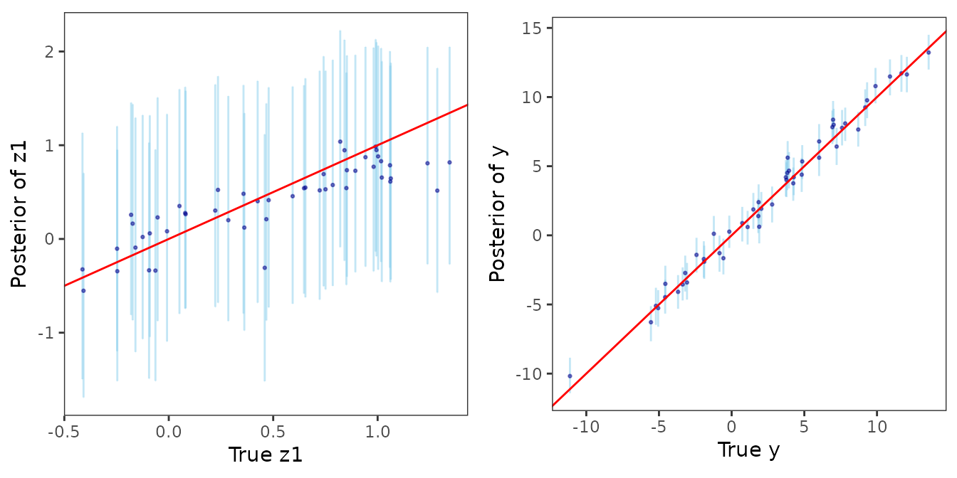
Prediction in spatial generalized linear model
Define the collection of candidate parameters and fit the model using
spGLMstack(). We use the Poisson counts y_pois
of simSpatial for this example.
# training and test data sizes
n_train <- 200
n_pred <- 50

dat_train <- simSpatial[1:n_train, ]
dat_pred <- simSpatial[n_train + 1:n_pred, ]

cand.mod <- candidateModels(list(phi = c(2, 4, 6, 8),
                                 nu = c(0.5, 1, 1.5, 1.75),
                                 boundary = c(0.5, 0.75)), "cartesian")

mod1 <- spGLMstack(y_pois ~ x1 + x2, data = dat_train, family = "poisson",
                   coords = as.matrix(dat_train[, c("s1", "s2")]), cor.fn = "matern",
                   candidate.models = cand.mod,
                   n.samples = 1000,
                   loopd.controls = list(method = "CV", CV.K = 10, nMC = 500),
                   verbose = TRUE)
##
## STACKING WEIGHTS:
##
## | phi | nu | boundary | weight |
## +----------+-----+------+----------+--------+
## | Model 1 | 2| 0.50| 0.50| 0.000 |
## | Model 2 | 4| 0.50| 0.50| 0.000 |
## | Model 3 | 6| 0.50| 0.50| 0.000 |
## | Model 4 | 8| 0.50| 0.50| 0.000 |
## | Model 5 | 2| 1.00| 0.50| 0.000 |
## | Model 6 | 4| 1.00| 0.50| 0.000 |
## | Model 7 | 6| 1.00| 0.50| 0.000 |
## | Model 8 | 8| 1.00| 0.50| 0.000 |
## | Model 9 | 2| 1.50| 0.50| 0.000 |
## | Model 10 | 4| 1.50| 0.50| 0.000 |
## | Model 11 | 6| 1.50| 0.50| 0.000 |
## | Model 12 | 8| 1.50| 0.50| 0.000 |
## | Model 13 | 2| 1.75| 0.50| 0.000 |
## | Model 14 | 4| 1.75| 0.50| 0.000 |
## | Model 15 | 6| 1.75| 0.50| 0.000 |
## | Model 16 | 8| 1.75| 0.50| 0.056 |
## | Model 17 | 2| 0.50| 0.75| 0.000 |
## | Model 18 | 4| 0.50| 0.75| 0.000 |
## | Model 19 | 6| 0.50| 0.75| 0.000 |
## | Model 20 | 8| 0.50| 0.75| 0.000 |
## | Model 21 | 2| 1.00| 0.75| 0.000 |
## | Model 22 | 4| 1.00| 0.75| 0.000 |
## | Model 23 | 6| 1.00| 0.75| 0.000 |
## | Model 24 | 8| 1.00| 0.75| 0.000 |
## | Model 25 | 2| 1.50| 0.75| 0.000 |
## | Model 26 | 4| 1.50| 0.75| 0.000 |
## | Model 27 | 6| 1.50| 0.75| 0.000 |
## | Model 28 | 8| 1.50| 0.75| 0.000 |
## | Model 29 | 2| 1.75| 0.75| 0.000 |
## | Model 30 | 4| 1.75| 0.75| 0.000 |
## | Model 31 | 6| 1.75| 0.75| 0.944 |
## | Model 32 | 8| 1.75| 0.75| 0.000 |
## +----------+-----+------+----------+--------+Define the new coordinates, run posteriorPredict(), and
finally sample from the stacked posterior. To demonstrate the
usage, we specify joint=FALSE for the prediction task.
sp_pred <- as.matrix(dat_pred[, c("s1", "s2")])
X_new <- cbind(1, dat_pred$x1, dat_pred$x2)
mod.pred <- posteriorPredict(mod1, coords_new = sp_pred, covars_new = X_new, joint = FALSE)
post_samps <- stackedSampler(mod.pred)
Finally, we analyze the posterior predictive distributions of the spatial process as well as the responses against their corresponding true values in order to assess how well the predictions are made.
postpred_z <- post_samps$z.pred
post_z_summ <- t(apply(postpred_z, 1, function(x) quantile(x, c(0.025, 0.5, 0.975))))
z_combn <- data.frame(z = dat_pred$z_true, zL = post_z_summ[, 1],
                      zM = post_z_summ[, 2], zU = post_z_summ[, 3])

plot_z_summ <- ggplot(data = z_combn, aes(x = z)) +
  geom_errorbar(aes(ymin = zL, ymax = zU), alpha = 0.5, color = "skyblue") +
  geom_point(aes(y = zM), size = 0.5, color = "darkblue", alpha = 0.5) +
  geom_abline(slope = 1, intercept = 0, color = "red", linetype = "solid") +
  xlab("True z") + ylab("Posterior predictive of z") + theme_bw() +
  theme(panel.grid = element_blank(), aspect.ratio = 1)

postpred_y <- post_samps$y.pred
post_y_summ <- t(apply(postpred_y, 1, function(x) quantile(x, c(0.025, 0.5, 0.975))))
y_combn <- data.frame(y = dat_pred$y_pois, yL = post_y_summ[, 1],
                      yM = post_y_summ[, 2], yU = post_y_summ[, 3])

plot_y_summ <- ggplot(data = y_combn, aes(x = y)) +
  geom_errorbar(aes(ymin = yL, ymax = yU), alpha = 0.5, color = "skyblue") +
  geom_point(aes(y = yM), size = 0.5, color = "darkblue", alpha = 0.5) +
  geom_abline(slope = 1, intercept = 0, color = "red", linetype = "solid") +
  xlab("True y") + ylab("Posterior predictive of y") + theme_bw() +
  theme(panel.grid = element_blank(), aspect.ratio = 1)

plot_z_summ + plot_y_summ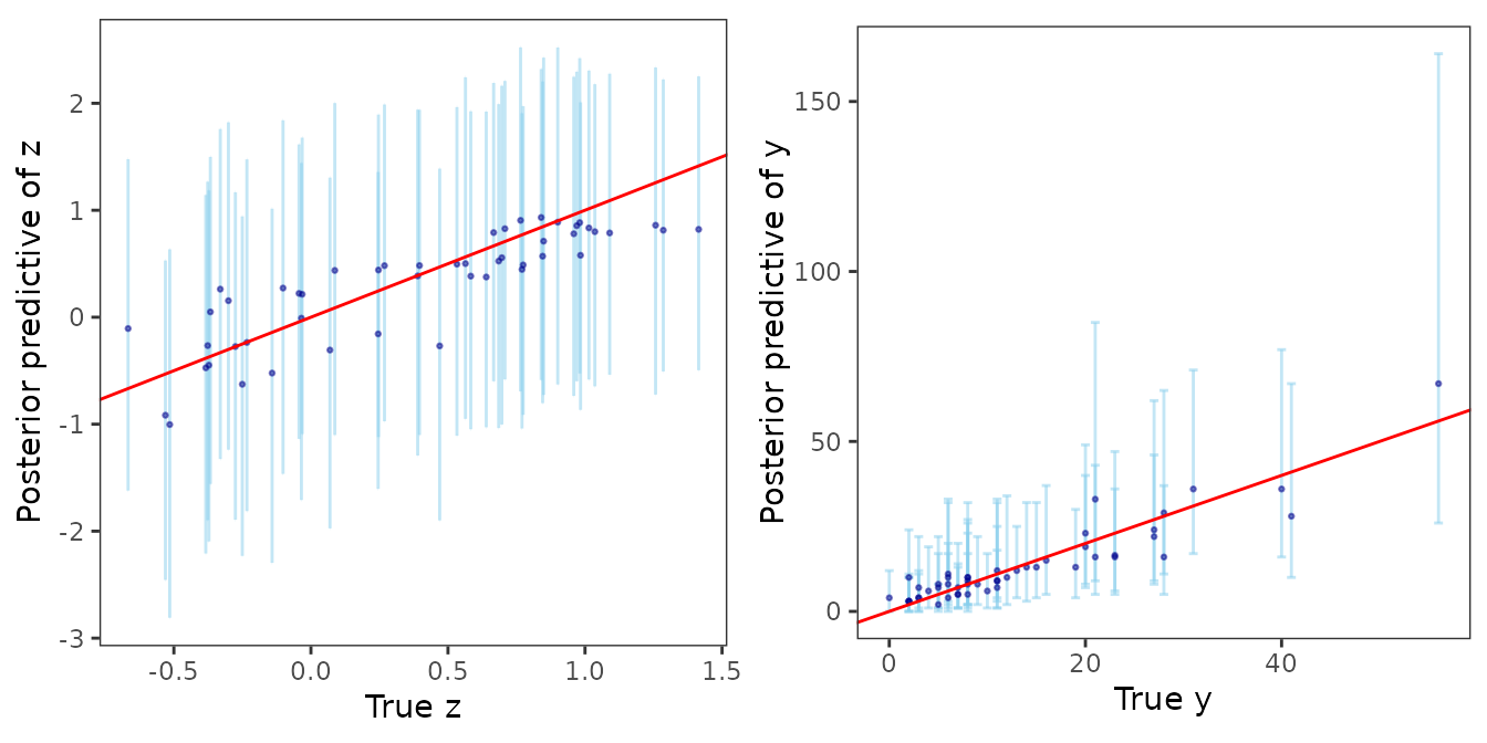
Prediction in spatially varying coefficients model
For the spatially varying coefficients models,
covars_new is a list with tags fixed
(covariates with fixed effects) and vc (covariates with
spatially varying coefficients), and coords_new is a matrix
of new coordinates as before. We fit svcLMstack() to the
Gaussian response y_svc of simSpatial, which
has a spatially varying intercept (z2_true) and a spatially
varying slope of x1 (5 + z_true).
n_train <- 200
n_pred <- 50
dat_train <- simSpatial[1:n_train, ]
dat_pred <- simSpatial[n_train + 1:n_pred, ]

cand.svc <- candidateModels(list(phi = list(c(4, 4), c(8, 4), c(8, 8)),
                                 nu = list(c(1.5, 1.5)),
                                 noise_sp_ratio = list(c(0.1, 0.1), c(0.25, 0.25))),
                            "cartesian")
mod_svc <- svcLMstack(y_svc ~ x1 + x2 + (x1), data = dat_train,
                      coords = as.matrix(dat_train[, c("s1", "s2")]),
                      cor.fn = "matern", process.type = "independent",
                      candidate.models = cand.svc,
                      n.samples = 1000, verbose = FALSE)

mod_svc_pred <- posteriorPredict(mod_svc,
                                 coords_new = as.matrix(dat_pred[, c("s1", "s2")]),
                                 covars_new = list(fixed = cbind(1, dat_pred$x1, dat_pred$x2),
                                                   vc = cbind(1, dat_pred$x1)),
                                 joint = TRUE)
post_samps <- stackedSampler(mod_svc_pred)
The rows
of z.pred hold the predicted varying intercept and the rows
the predicted varying part of the slope of x1.
plot_pred <- function(truth, samps, lab){
  summ <- t(apply(samps, 1, function(x) quantile(x, c(0.025, 0.5, 0.975))))
  df <- data.frame(truth = truth, L = summ[, 1], M = summ[, 2], U = summ[, 3])
  ggplot(data = df, aes(x = truth)) +
    geom_errorbar(aes(ymin = L, ymax = U), alpha = 0.5, color = "skyblue") +
    geom_point(aes(y = M), size = 0.5, color = "darkblue", alpha = 0.5) +
    geom_abline(slope = 1, intercept = 0, color = "red", linetype = "solid") +
    xlab(paste("True", lab)) + ylab(paste("Posterior predictive of", lab)) +
    theme_bw() + theme(panel.grid = element_blank(), aspect.ratio = 1)
}
plot_pred(dat_pred$z2_true, post_samps$z.pred[1:n_pred, ], "z0") +
  plot_pred(dat_pred$z_true, post_samps$z.pred[n_pred + 1:n_pred, ], "z1") +
  plot_pred(dat_pred$y_svc, post_samps$y.pred, "y")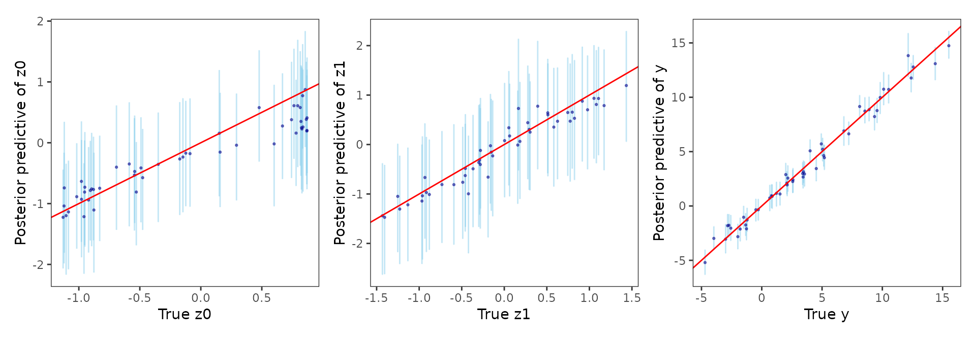
Prediction in spatially-temporally varying coefficients model
Define the collection of candidate parameters and fit the model using
stvcGLMstack(). We use the Poisson counts
y_pois of simSpaceTime for this example.
# Example 2: Spatial-temporal model with varying coefficients
n_train <- 300
n_pred <- 50
data("simSpaceTime")

# split dataset into test and train
dat_train <- simSpaceTime[1:n_train, ]
dat_pred <- simSpaceTime[n_train + 1:n_pred, ]

# create list of candidate models (multivariate)
mod.list2 <- candidateModels(list(phi_s = list(2, 3, 4),
                                  phi_t = list(2, 4, 8),
                                  boundary = c(0.5, 0.75)), "cartesian")

# fit a spatial-temporal varying coefficient model using predictive stacking
mod1 <- stvcGLMstack(y_pois ~ x1 + x2 + (x1), data = dat_train, family = "poisson",
                     sp_coords = as.matrix(dat_train[, c("s1", "s2")]),
                     time_coords = as.matrix(dat_train[, "t_coords"]),
                     cor.fn = "gneiting-decay",
                     process.type = "multivariate",
                     candidate.models = mod.list2,
                     loopd.controls = list(method = "CV", CV.K = 10, nMC = 500),
                     n.samples = 500)
##
## STACKING WEIGHTS:
##
## | phi_s | phi_t | boundary | weight |
## +----------+-------+-------+----------+--------+
## | Model 1 | 2| 2| 0.50| 0 |
## | Model 2 | 3| 2| 0.50| 0 |
## | Model 3 | 4| 2| 0.50| 0 |
## | Model 4 | 2| 4| 0.50| 0 |
## | Model 5 | 3| 4| 0.50| 0 |
## | Model 6 | 4| 4| 0.50| 0 |
## | Model 7 | 2| 8| 0.50| 0 |
## | Model 8 | 3| 8| 0.50| 0 |
## | Model 9 | 4| 8| 0.50| 0 |
## | Model 10 | 2| 2| 0.75| 0 |
## | Model 11 | 3| 2| 0.75| 0 |
## | Model 12 | 4| 2| 0.75| 0 |
## | Model 13 | 2| 4| 0.75| 1 |
## | Model 14 | 3| 4| 0.75| 0 |
## | Model 15 | 4| 4| 0.75| 0 |
## | Model 16 | 2| 8| 0.75| 0 |
## | Model 17 | 3| 8| 0.75| 0 |
## | Model 18 | 4| 8| 0.75| 0 |
## +----------+-------+-------+----------+--------+Define the new coordinates, run posteriorPredict(), and
finally sample from the stacked posterior. We use
joint=FALSE for this particular example.
# prepare new coordinates and covariates for prediction
sp_pred <- as.matrix(dat_pred[, c("s1", "s2")])
tm_pred <- as.matrix(dat_pred[, "t_coords"])
X_new <- cbind(1, dat_pred$x1, dat_pred$x2)     # covariates with fixed effects
XTilde_new <- cbind(1, dat_pred$x1)              # covariates with varying coefficients
mod_pred <- posteriorPredict(mod1,
                             coords_new = list(sp = sp_pred, time = tm_pred),
                             covars_new = list(fixed = X_new, vc = XTilde_new),
                             joint = FALSE)

# sample from the stacked posterior and posterior predictive distribution
post_samps <- stackedSampler(mod_pred)
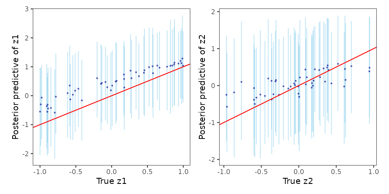
Finally, we analyze the posterior predictive distributions of the spatial-temporal process by plotting them against their corresponding true values.
postpred_z <- post_samps$z.pred
post_z1_summ <- t(apply(postpred_z[1:n_pred,], 1,
                        function(x) quantile(x, c(0.025, 0.5, 0.975))))
post_z2_summ <- t(apply(postpred_z[n_pred + 1:n_pred,], 1,
                        function(x) quantile(x, c(0.025, 0.5, 0.975))))

z1_combn <- data.frame(z = dat_pred$z1_true, zL = post_z1_summ[, 1],
                       zM = post_z1_summ[, 2], zU = post_z1_summ[, 3])
z2_combn <- data.frame(z = dat_pred$z2_true, zL = post_z2_summ[, 1],
                       zM = post_z2_summ[, 2], zU = post_z2_summ[, 3])

plot_z1_summ <- ggplot(data = z1_combn, aes(x = z)) +
  geom_errorbar(aes(ymin = zL, ymax = zU), alpha = 0.5, color = "skyblue") +
  geom_point(aes(y = zM), size = 0.5, color = "darkblue", alpha = 0.5) +
  geom_abline(slope = 1, intercept = 0, color = "red", linetype = "solid") +
  xlab("True z1") + ylab("Posterior predictive of z1") + theme_bw() +
  theme(panel.grid = element_blank(), aspect.ratio = 1)

plot_z2_summ <- ggplot(data = z2_combn, aes(x = z)) +
  geom_errorbar(aes(ymin = zL, ymax = zU), alpha = 0.5, color = "skyblue") +
  geom_point(aes(y = zM), size = 0.5, color = "darkblue", alpha = 0.5) +
  geom_abline(slope = 1, intercept = 0, color = "red", linetype = "solid") +
  xlab("True z2") + ylab("Posterior predictive of z2") + theme_bw() +
  theme(panel.grid = element_blank(), aspect.ratio = 1)

plot_z1_summ + plot_z2_summ