In this article, we discuss the following functions -
These functions can be used to fit Gaussian and non-Gaussian spatial point-referenced data.
set.seed(1729)Bayesian Gaussian spatial regression models
In this section, we thoroughly illustrate our method on synthetic Gaussian as well as non-Gaussian spatial data and provide code to analyze the output of our functions. We start by loading the package.
Some synthetic spatial data are lazy-loaded which includes synthetic
spatial Gaussian data simGaussian, Poisson data
simPoisson, binomial data simBinom and binary
data simBinary. One can use the function
sim_spData() to simulate spatial data. We will be applying
our functions on these datasets.
Using fixed hyperparameters
We first load the data simGaussian and set up the
priors. Supplying the priors is optional. See the documentation of
spLMexact() to learn more about the default priors.
Besides, setting the priors, we also fix the values of the spatial
process parameters (spatial decay
and smoothness
)
and the noise-to-spatial variance ratio
().
data("simGaussian")
dat <- simGaussian[1:200, ] # work with first 200 rows

muBeta <- c(0, 0)
VBeta <- cbind(c(1E4, 0.0), c(0.0, 1E4))
sigmaSqIGa <- 2
sigmaSqIGb <- 2
phi0 <- 3
nu0 <- 0.5
noise_sp_ratio <- 0.8
prior_list <- list(beta.norm = list(muBeta, VBeta),
                   sigma.sq.ig = c(sigmaSqIGa, sigmaSqIGb))
nSamples <- 1000
We define the spatial model using a formula, similar to
that in the widely used lm() function in the
stats package. Here, the formula y ~ x1
corresponds to the spatial linear model
where the y corresponds to the response variable
,
which is regressed on the predictor x1 given by
.
The intercept is automatically considered within the model, and hence
y ~ x1 is functionally equivalent to
y ~ 1 + x1. Moreover, a spatial random effect is inherent
in the model, where the spatial correlation matrix is governed by the
spatial correlation function specified by the argument
cor.fn. Supported correlation functions are
"exponential" and "matern". The exponential
covariogram is specified by the hyperparameter
and the Matern covariogram is specified by the hyperparameters
and
.
Fixed values of these hyperparameters are supplied through the argument
spParams. In addition, the noise-to-spatial variance ration
is also fixed through the argument noise_sp_ratio.
If interested in calculation of leave-one-out predictive densities
(LOO-PD), loopd must be set TRUE (the default
is FALSE). Method of LOO-PD calculation can be also set by
the option loopd.method which support the keywords
"exact" and "psis". The option
"exact" exploits the analytically available expressions of
the predictive density and implements an efficient row-deletion Cholesky
factor update for fast calculation and avoids refitting the model
times, where
is the sample size. On the other hand, "psis" implements
Pareto-smoothed importance sampling and finds approximate LOO-PD and is
much faster than "exact".
We pass these arguments into the function
spLMexact().
mod1 <- spLMexact(y ~ x1, data = dat,
                  coords = as.matrix(dat[, c("s1", "s2")]),
                  cor.fn = "matern",
                  priors = prior_list,
                  spParams = list(phi = phi0, nu = nu0),
                  noise_sp_ratio = noise_sp_ratio, n.samples = nSamples,
                  loopd = TRUE, loopd.method = "exact",
                  verbose = TRUE)
#> ----------------------------------------
#>  Model description
#> ----------------------------------------
#> Model fit with 200 observations.
#>
#> Number of covariates 2 (including intercept).
#>
#> Using the matern spatial correlation function.
#>
#> Priors:
#>  beta: Gaussian
#>  mu: 0.00    0.00
#>  cov:
#>   10000.00    0.00
#>   0.00    10000.00
#>
#>  sigma.sq: Inverse-Gamma
#>  shape = 2.00, scale = 2.00.
#>
#> Spatial process parameters:
#>  phi = 3.00, and, nu = 0.50.
#> Noise-to-spatial variance ratio = 0.80.
#>
#> Number of posterior samples = 1000.
#>
#> LOO-PD calculation method = exact.
#> ----------------------------------------
Next, we can summarize the posterior samples of the fixed effects as follows.
Leave-one-out predictive densities using PSIS
Out of curiosity, we find the LOO-PD for the same model using the approximate method that uses Pareto-smoothed importance sampling, or PSIS. See Vehtari, Gelman, and Gabry (2017) for details.
mod2 <- spLMexact(y ~ x1, data = dat,
                  coords = as.matrix(dat[, c("s1", "s2")]),
                  cor.fn = "matern",
                  priors = prior_list,
                  spParams = list(phi = phi0, nu = nu0),
                  noise_sp_ratio = noise_sp_ratio, n.samples = nSamples,
                  loopd = TRUE, loopd.method = "PSIS",
                  verbose = FALSE)
Subsquently, we compare the LOO-PD obtained by the two methods.
loopd_exact <- mod1$loopd
loopd_psis <- mod2$loopd
loopd_df <- data.frame(exact = loopd_exact, psis = loopd_psis)

library(ggplot2)
plot1 <- ggplot(data = loopd_df, aes(x = exact)) +
  geom_point(aes(y = psis), size = 1, alpha = 0.5) +
  geom_abline(slope = 1, intercept = 0, color = "red", alpha = 0.5) +
  xlab("Exact") + ylab("PSIS") + theme_bw() +
  theme(panel.background = element_blank(),
        panel.grid = element_blank(), aspect.ratio = 1)
plot1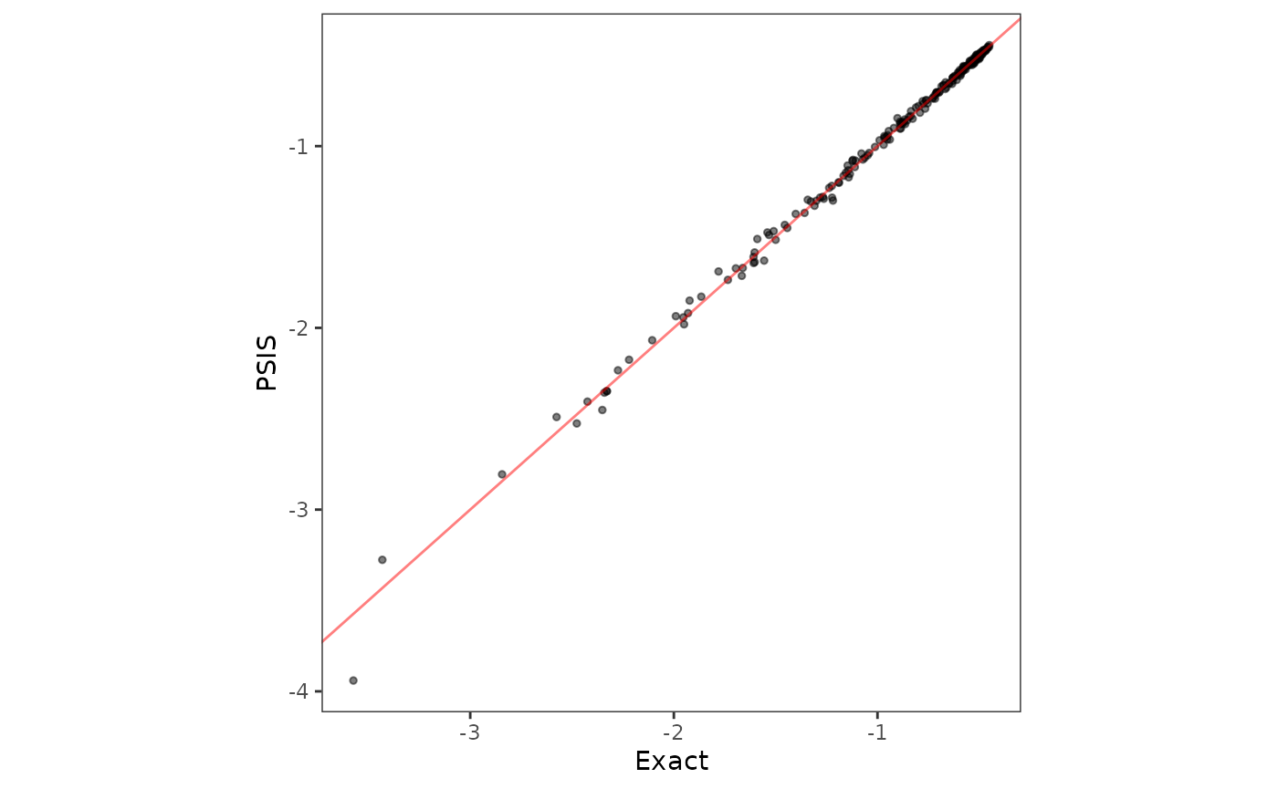
Using predictive stacking
Next, we move on to the Bayesian spatial stacking algorithm for Gaussian data. We supply the same prior list and provide some candidate values of spatial process parameters and noise-to-spatial variance ratio.
mod3 <- spLMstack(y ~ x1, data = dat,
                  coords = as.matrix(dat[, c("s1", "s2")]),
                  cor.fn = "matern",
                  priors = prior_list,
                  params.list = list(phi = c(1.5, 3, 5),
                                     nu = c(0.5, 1, 1.5),
                                     noise_sp_ratio = c(0.5, 1.5)),
                  n.samples = 1000, loopd.method = "exact",
                  parallel = FALSE, verbose = TRUE)
#> --------------------------------------------------
#> Solver diagnostics:
#> Installed solvers: CLARABEL, SCS, OSQP, HIGHS
#> Requested solver: DEFAULT (CLARABEL -> ECOS -> SCS)
#> Solver search order: CLARABEL -> SCS
#> --------------------------------------------------
#> ────────────────────────────────── CVXR v1.8.1 ─────────────────────────────────
#> ℹ Problem: 1 variable, 2 constraints (DCP)
#> ℹ Compilation: "CLARABEL" via CVXR::FlipObjective -> CVXR::Dcp2Cone -> CVXR::CvxAttr2Constr -> CVXR::ConeMatrixStuffing -> CVXR::Clarabel_Solver
#> ℹ Compile time: 0.923s
#> ─────────────────────────────── Numerical solver ───────────────────────────────
#> ──────────────────────────────────── Summary ───────────────────────────────────
#> ✔ Status: optimal
#> ✔ Optimal value: -113.076
#> ℹ Compile time: 0.923s
#> ℹ Solver time: 0.031s
#>
#> STACKING WEIGHTS:
#>
#>            | phi | nu  | noise_sp_ratio | weight |
#> +----------+-----+-----+----------------+--------+
#> | Model 1  |  1.5|  0.5|             0.5| 0.000  |
#> | Model 2  |  3.0|  0.5|             0.5| 0.000  |
#> | Model 3  |  5.0|  0.5|             0.5| 0.000  |
#> | Model 4  |  1.5|  1.0|             0.5| 0.242  |
#> | Model 5  |  3.0|  1.0|             0.5| 0.000  |
#> | Model 6  |  5.0|  1.0|             0.5| 0.751  |
#> | Model 7  |  1.5|  1.5|             0.5| 0.000  |
#> | Model 8  |  3.0|  1.5|             0.5| 0.000  |
#> | Model 9  |  5.0|  1.5|             0.5| 0.000  |
#> | Model 10 |  1.5|  0.5|             1.5| 0.000  |
#> | Model 11 |  3.0|  0.5|             1.5| 0.000  |
#> | Model 12 |  5.0|  0.5|             1.5| 0.000  |
#> | Model 13 |  1.5|  1.0|             1.5| 0.000  |
#> | Model 14 |  3.0|  1.0|             1.5| 0.000  |
#> | Model 15 |  5.0|  1.0|             1.5| 0.006  |
#> | Model 16 |  1.5|  1.5|             1.5| 0.000  |
#> | Model 17 |  3.0|  1.5|             1.5| 0.000  |
#> | Model 18 |  5.0|  1.5|             1.5| 0.000  |
#> +----------+-----+-----+----------------+--------+
The user can check the solver status and runtime by issuing the following.
Analyzing samples from the stacked posterior
To sample from the stacked posterior, the package provides a helper
function called stackedSampler(). Subsequent inference
proceeds from these samples obtained from the stacked posterior.
post_samps <- stackedSampler(mod3)We then collect the samples of the fixed effects and summarize them as follows.
post_beta <- post_samps$beta
summary_beta <- t(apply(post_beta, 1, function(x) quantile(x, c(0.025, 0.5, 0.975))))
rownames(summary_beta) <- mod3$X.names
print(summary_beta)
#>                  2.5%      50%    97.5%
#> (Intercept) 0.9540551 2.220069 3.057419
#> x1          4.8672400 4.949081 5.036638
The synthetic data simGaussian was simulated using the
true value
.
We notice that the stacked posterior is concentrated around the
truth.
library(tidyr)
library(dplyr)
#>
#> Attaching package: 'dplyr'
#> The following objects are masked from 'package:stats':
#>
#>     filter, lag
#> The following objects are masked from 'package:base':
#>
#>     intersect, setdiff, setequal, union

post_beta_df <- as.data.frame(post_beta)
post_beta_df <- post_beta_df %>%
  mutate(row = paste0("beta", row_number()-1)) %>%
  pivot_longer(-row, names_to = "sample", values_to = "value")

# True values of beta0 and beta1
truth <- data.frame(row = c("beta0", "beta1"), true_value = c(2, 5))

ggplot(post_beta_df, aes(x = value)) +
  geom_density(fill = "lightblue", alpha = 0.6) +
  geom_vline(data = truth, aes(xintercept = true_value),
             color = "red", linetype = "dashed", linewidth = 0.5) +
  facet_wrap(~ row, scales = "free") + labs(x = "", y = "Density") +
  theme_bw() + theme(panel.background = element_blank(),
                     panel.grid = element_blank(), aspect.ratio = 1)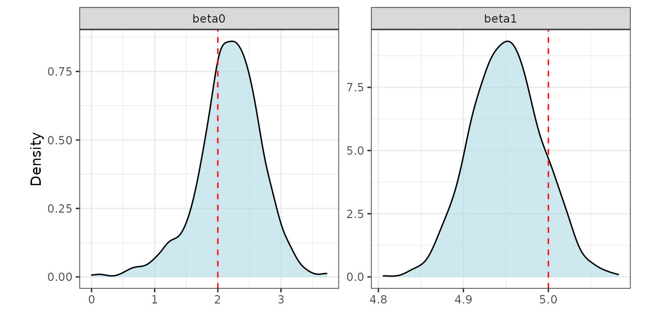
Furthermore, we compare the posterior samples of the spatial random effects with their corresponding true values.
post_z <- post_samps$z
post_z_summ <- t(apply(post_z, 1, function(x) quantile(x, c(0.025, 0.5, 0.975))))
z_combn <- data.frame(z = dat$z_true, zL = post_z_summ[, 1],
                      zM = post_z_summ[, 2], zU = post_z_summ[, 3])

plotz <- ggplot(data = z_combn, aes(x = z)) +
  geom_point(aes(y = zM), size = 0.75, color = "darkblue", alpha = 0.5) +
  geom_errorbar(aes(ymin = zL, ymax = zU), width = 0.05, alpha = 0.15,
                color = "skyblue") +
  geom_abline(slope = 1, intercept = 0, color = "red") +
  xlab("True z") + ylab("Stacked posterior of z") + theme_bw() +
  theme(panel.background = element_blank(),
        panel.grid = element_blank(), aspect.ratio = 1)
plotz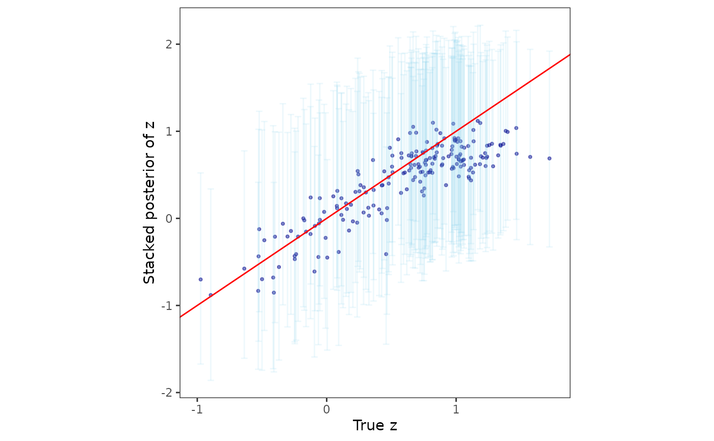
The package also provides helper functions to plot interpolated
spatial surfaces in order for visualization purposes. The function
surfaceplot() creates a single spatial surface plot, while
surfaceplot2() creates two side-by-side surface plots. We
are using the later to visually inspect the interpolated spatial
surfaces of the true spatial effects and their posterior medians.
postmedian_z <- apply(post_z, 1, median)
dat$z_hat <- postmedian_z
plot_z <- surfaceplot2(dat, coords_name = c("s1", "s2"),
                       var1_name = "z_true", var2_name = "z_hat")
#> Warning: `aes_string()` was deprecated in ggplot2 3.0.0.
#> ℹ Please use tidy evaluation idioms with `aes()`.
#> ℹ See also `vignette("ggplot2-in-packages")` for more information.
#> ℹ The deprecated feature was likely used in the spStack package.
#>   Please report the issue at <https://github.com/SPan-18/spStack-dev/issues>.
#> This warning is displayed once per session.
#> Call `lifecycle::last_lifecycle_warnings()` to see where this warning was
#> generated.
patchwork::wrap_plots(plot_z) +
    patchwork::plot_layout(guides = "collect") &
    ggplot2::theme(legend.position = "right")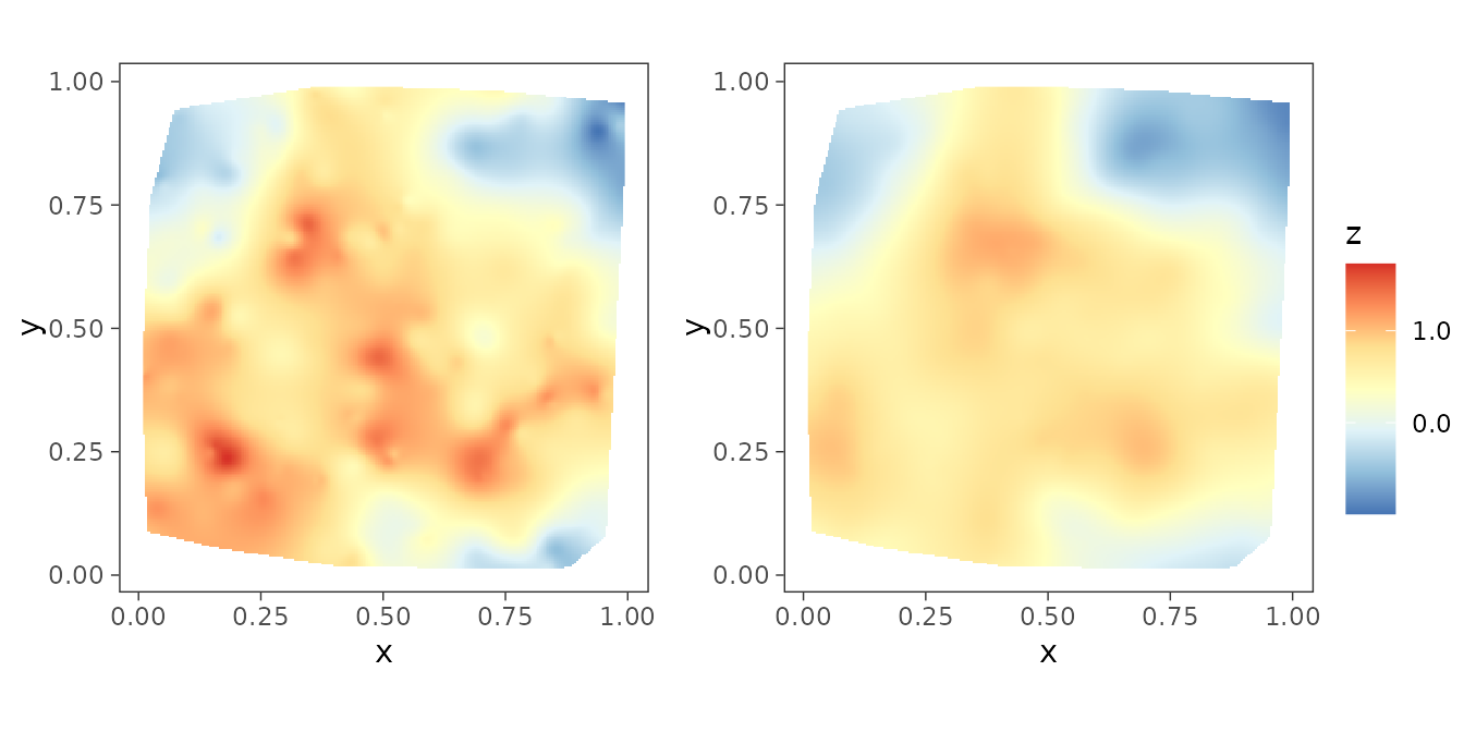
Analysis of spatial non-Gaussian data
We also offer functions for Bayesian analysis of spatially point-referenced Poisson, binomial count, and binary data.
Spatial Poisson count data
We first load and plot the point-referenced Poisson count data.
data("simPoisson")
dat <- simPoisson[1:200, ] # work with first 200 observations

ggplot(dat, aes(x = s1, y = s2)) +
  geom_point(aes(color = y), alpha = 0.75) +
  scale_color_distiller(palette = "RdYlGn", direction = -1,
                        label = function(x) sprintf("%.0f", x)) +
  guides(alpha = 'none') + theme_bw() +
  theme(axis.ticks = element_line(linewidth = 0.25),
        panel.background = element_blank(), panel.grid = element_blank(),
        legend.title = element_text(size = 10, hjust = 0.25),
        legend.box.just = "center", aspect.ratio = 1)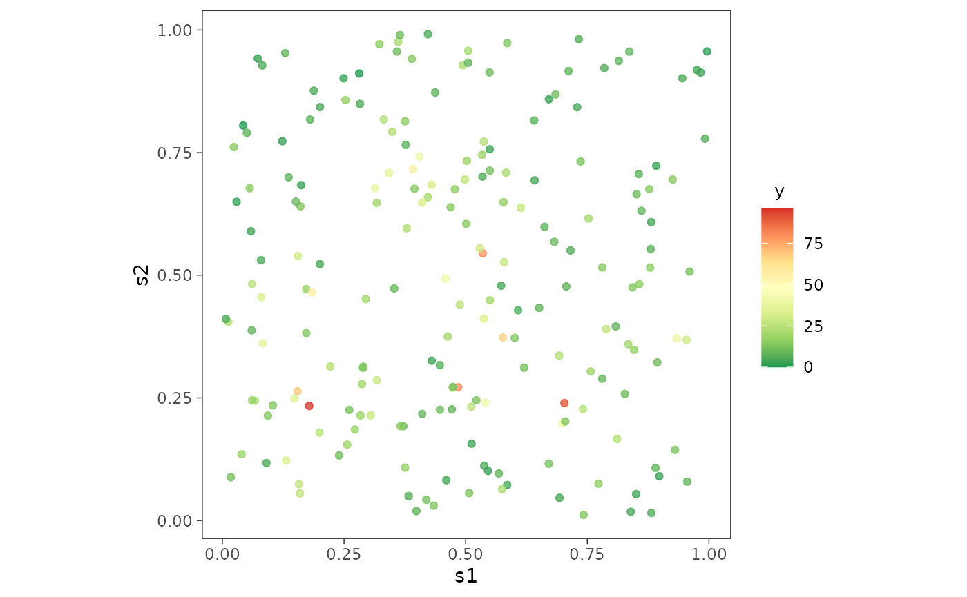
Under fixed hyperparameters
Next, we demonstrate the function spGLMexact() which
delivers posterior samples of the fixed effects and the spatial random
effects. The option family must be specified correctly
while using this function. For instance, in the following example, the
formula y ~ x1 and family = "poisson"
corresponds to the spatial regression model
We provide fixed values of the spatial process parameters and a
boundary adjustment parameter, given by the argument
boundary, which if not supplied, defaults to 0.5. For
details on the priors and its default value, see function
documentation.
mod1 <- spGLMexact(y ~ x1, data = dat, family = "poisson",
                   coords = as.matrix(dat[, c("s1", "s2")]), cor.fn = "matern",
                   spParams = list(phi = phi0, nu = nu0),
                   priors = list(nu.beta = 5, nu.z = 5),
                   boundary = 0.5,
                   n.samples = 1000, verbose = TRUE)
#> Some priors were not supplied. Using defaults.
#> ----------------------------------------
#>  Model description
#> ----------------------------------------
#> Model fit with 200 observations.
#>
#> Family = poisson.
#>
#> Number of covariates 2 (including intercept).
#>
#> Using the matern spatial correlation function.
#>
#> Priors:
#>  beta: Gaussian
#>  mu: 0.00    0.00
#>  cov:
#>   100.00  0.00
#>   0.00    100.00
#>
#>  sigmaSq.beta ~ IG(nu.beta/2, nu.beta/2)
#>  sigmaSq.z ~ IG(nu.z/2, nu.z/2)
#>  nu.beta = 5.00, nu.z = 5.00.
#>  sigmaSq.xi = 0.10.
#>  Boundary adjustment parameter = 0.50.
#>
#> Spatial process parameters:
#>  phi = 3.00, and, nu = 0.50.
#>
#> Number of posterior samples = 1000.
#> ----------------------------------------
We next collect the samples of the fixed effects and summarize them.
The true value of the fixed effects with which the data was simulated is
(for more details, see the documentation of the data
simPoisson).
Posterior recovery of scale parameters
The analytic tractability of the posterior distribution under the
framework is enabled by marginalizing out the scale parameters
and
associated with the fixed effects
and the spatial random effects
,
respectively. However, posterior samples of
and
can be recovered using the function recoverGLMscale().
mod1 <- recoverGLMscale(mod1)We visualize the posterior distributions of and through histograms.
post_scale_df <- data.frame(value = sqrt(c(mod1$samples$sigmasq.beta, mod1$samples$sigmasq.z)),
                            group = factor(rep(c("sigma.beta", "sigma.z"),
                                    each = length(mod1$samples$sigmasq.beta))))
ggplot(post_scale_df, aes(x = value)) +
  geom_density(fill = "lightblue", alpha = 0.6) +
  facet_wrap(~ group, scales = "free") + labs(x = "", y = "Density") +
  theme_bw() + theme(panel.background = element_blank(),
                     panel.grid = element_blank(), aspect.ratio = 1)
Using predictive stacking
Next, we move on to the function spGLMstack() that will
implement our proposed stacking algorithm. The argument
loopd.controls is used to provide details on what algorithm
to be used to find LOO-PD. Valid options for the tag method
is "exact" and "CV". We use
-fold
cross-validation by assigning method = "CV"and
CV.K = 10. The tag nMC decides the number of
Monte Carlo samples to be used to find the LOO-PD.
mod2 <- spGLMstack(y ~ x1, data = dat, family = "poisson",
                   coords = as.matrix(dat[, c("s1", "s2")]), cor.fn = "matern",
                   params.list = list(phi = c(3, 7, 10), nu = c(0.5, 1.5),
                                      boundary = c(0.5, 0.6)),
                   n.samples = 1000, priors = list(mu.beta = 5, nu.z = 5),
                   loopd.controls = list(method = "CV", CV.K = 10, nMC = 1000),
                   parallel = TRUE, verbose = TRUE)
#> Some priors were not supplied. Using defaults.
#> --------------------------------------------------
#> Solver diagnostics:
#> Installed solvers: CLARABEL, SCS, OSQP, HIGHS
#> Requested solver: DEFAULT (CLARABEL -> ECOS -> SCS)
#> Solver search order: CLARABEL -> SCS
#> --------------------------------------------------
#> ────────────────────────────────── CVXR v1.8.1 ─────────────────────────────────
#> ℹ Problem: 1 variable, 2 constraints (DCP)
#> ℹ Compilation: "CLARABEL" via CVXR::FlipObjective -> CVXR::Dcp2Cone -> CVXR::CvxAttr2Constr -> CVXR::ConeMatrixStuffing -> CVXR::Clarabel_Solver
#> ℹ Compile time: 0.191s
#> ─────────────────────────────── Numerical solver ───────────────────────────────
#> ──────────────────────────────────── Summary ───────────────────────────────────
#> ✔ Status: optimal
#> ✔ Optimal value: -311.489
#> ℹ Compile time: 0.191s
#> ℹ Solver time: 0.045s
#>
#> STACKING WEIGHTS:
#>
#>            | phi | nu  | boundary | weight |
#> +----------+-----+-----+----------+--------+
#> | Model 1  |    3|  0.5|       0.5| 0.000  |
#> | Model 2  |    7|  0.5|       0.5| 0.000  |
#> | Model 3  |   10|  0.5|       0.5| 0.000  |
#> | Model 4  |    3|  1.5|       0.5| 0.000  |
#> | Model 5  |    7|  1.5|       0.5| 0.000  |
#> | Model 6  |   10|  1.5|       0.5| 0.000  |
#> | Model 7  |    3|  0.5|       0.6| 0.000  |
#> | Model 8  |    7|  0.5|       0.6| 0.000  |
#> | Model 9  |   10|  0.5|       0.6| 0.000  |
#> | Model 10 |    3|  1.5|       0.6| 0.005  |
#> | Model 11 |    7|  1.5|       0.6| 0.724  |
#> | Model 12 |   10|  1.5|       0.6| 0.272  |
#> +----------+-----+-----+----------+--------+
We can extract information on solver status and runtime by the following.
print(mod2$solver)
#> [1] "CVXR:CLARABEL"
print(mod2$solver.status)
#> [1] "optimal"
print(mod2$run.time)
#>    user  system elapsed
#>  35.112  25.120  15.414
Further, we can recover the posterior samples of the scale parameters
by passing the output obtained by running spGLMstack() once
again through recoverGLMscale().
mod2 <- recoverGLMscale(mod2)Sampling from stacked posterior
We first obtain final posterior samples by sampling from the stacked sampler.
post_samps <- stackedSampler(mod2)Subsequently, we summarize the posterior samples of the fixed effects.
post_beta <- post_samps$beta
summary_beta <- t(apply(post_beta, 1, function(x) quantile(x, c(0.025, 0.5, 0.975))))
rownames(summary_beta) <- mod3$X.names
print(summary_beta)
#>                   2.5%        50%      97.5%
#> (Intercept)  1.1209791  2.1014709  3.0766891
#> x1          -0.6233661 -0.5472512 -0.4717314
The synthetic data simPoisson was simulated using
.
post_beta_df <- as.data.frame(post_beta)
post_beta_df <- post_beta_df %>%
  mutate(row = paste0("beta", row_number()-1)) %>%
  pivot_longer(-row, names_to = "sample", values_to = "value")

# True values of beta0 and beta1
truth <- data.frame(row = c("beta0", "beta1"), true_value = c(2, -0.5))

ggplot(post_beta_df, aes(x = value)) +
  geom_density(fill = "lightblue", alpha = 0.6) +
  geom_vline(data = truth, aes(xintercept = true_value),
             color = "red", linetype = "dashed", linewidth = 0.5) +
  facet_wrap(~ row, scales = "free") + labs(x = "", y = "Density") +
  theme_bw() + theme(panel.background = element_blank(),
                     panel.grid = element_blank(), aspect.ratio = 1)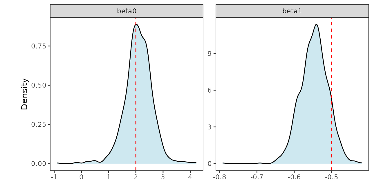
Finally, we analyze the posterior samples of the spatial random effects.
post_z <- post_samps$z
post_z_summ <- t(apply(post_z, 1, function(x) quantile(x, c(0.025, 0.5, 0.975))))
z_combn <- data.frame(z = dat$z_true, zL = post_z_summ[, 1],
                      zM = post_z_summ[, 2], zU = post_z_summ[, 3])

plotz <- ggplot(data = z_combn, aes(x = z)) +
  geom_point(aes(y = zM), size = 0.75, color = "darkblue", alpha = 0.5) +
  geom_errorbar(aes(ymin = zL, ymax = zU), width = 0.05, alpha = 0.15,
                color = "skyblue") +
  geom_abline(slope = 1, intercept = 0, color = "red") +
  xlab("True z") + ylab("Stacked posterior of z") + theme_bw() +
  theme(panel.background = element_blank(),
        panel.grid = element_blank(), aspect.ratio = 1)
plotz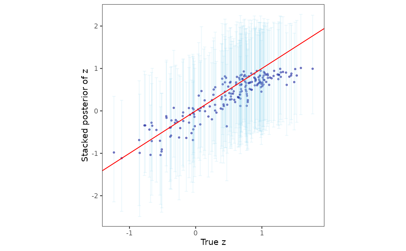
We can also compare the interpolated spatial surfaces of the true spatial effects with that of their posterior median.
postmedian_z <- apply(post_z, 1, median)
dat$z_hat <- postmedian_z
plot_z <- surfaceplot2(dat, coords_name = c("s1", "s2"),
                       var1_name = "z_true", var2_name = "z_hat")
patchwork::wrap_plots(plot_z) +
    patchwork::plot_layout(guides = "collect") &
    ggplot2::theme(legend.position = "right")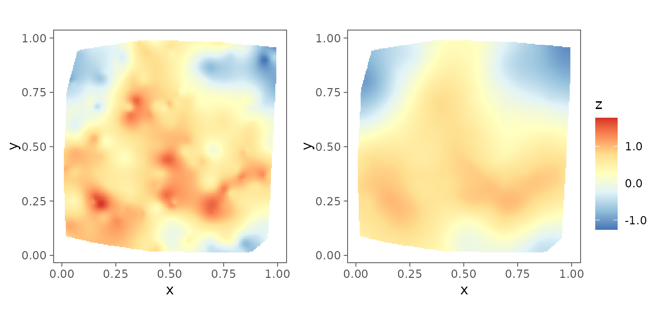
Spatial binomial count data
This will follow the same workflow as Poisson data with the exception
that the structure of formula that defines the model will
also contain the total number of trials at each location. Here, we
present only the spGLMexact() function for brevity.
data("simBinom")
dat <- simBinom[1:200, ] # work with first 200 rows

mod1 <- spGLMexact(cbind(y, n_trials) ~ x1, data = dat, family = "binomial",
                   coords = as.matrix(dat[, c("s1", "s2")]), cor.fn = "matern",
                   spParams = list(phi = 3, nu = 0.5),
                   boundary = 0.5, n.samples = 1000, verbose = FALSE)
Similarly, we collect the posterior samples of the fixed effects and summarize them. The true value of the fixed effects with which the data was simulated is .
Spatial binary data
Finally, we present only the spGLMexact() function for
spatial binary data to avoid repetition. In this case, unlike the
binomial model, almost nothing changes from that of in the case of
spatial Poisson data.
data("simBinary")
dat <- simBinary[1:200, ]

mod1 <- spGLMexact(y ~ x1, data = dat, family = "binary",
                   coords = as.matrix(dat[, c("s1", "s2")]), cor.fn = "matern",
                   spParams = list(phi = 4, nu = 0.4),
                   boundary = 0.5, n.samples = 1000, verbose = FALSE)
Similarly, we collect the posterior samples of the fixed effects and summarize them. The true value of the fixed effects with which the data was simulated is .