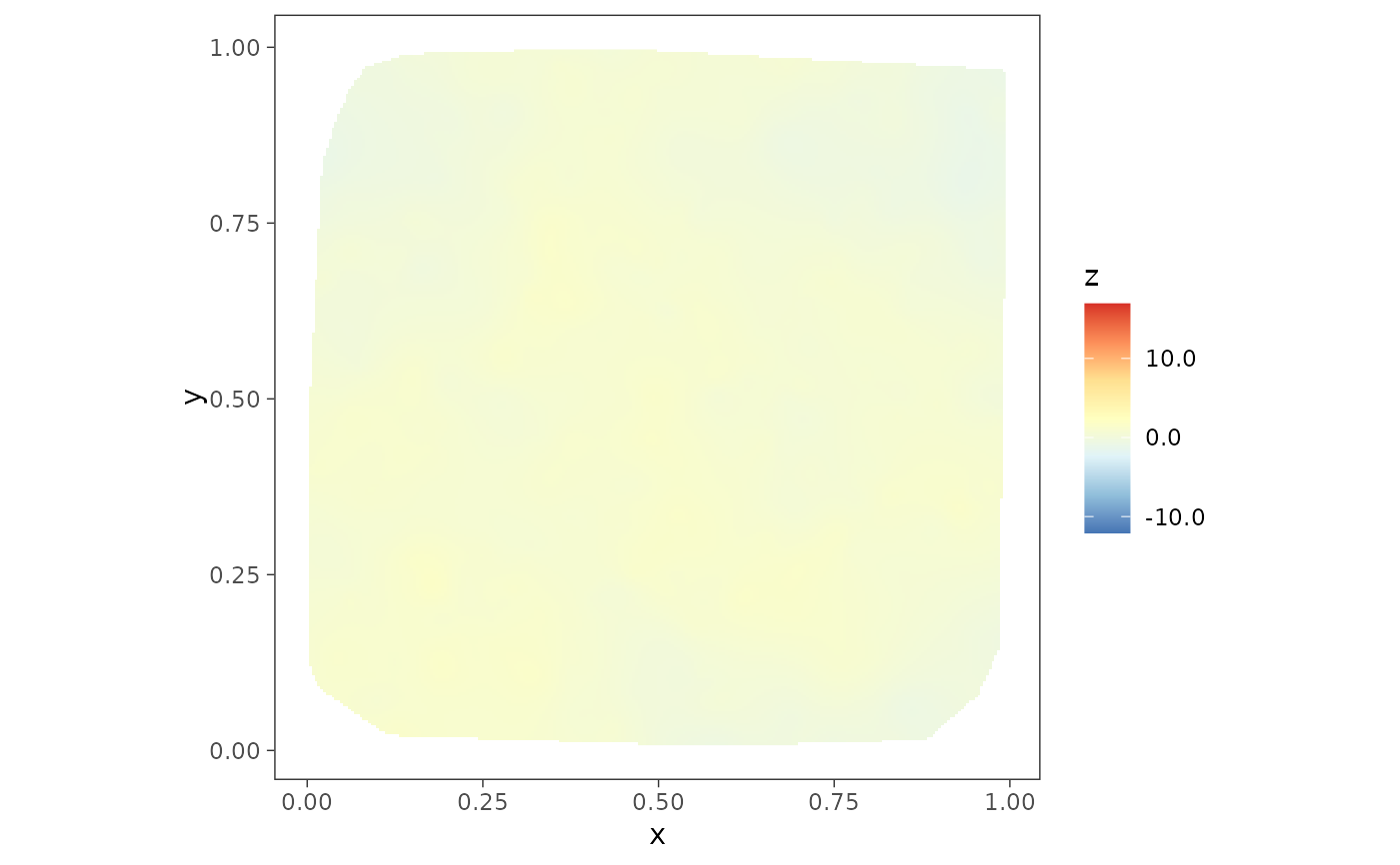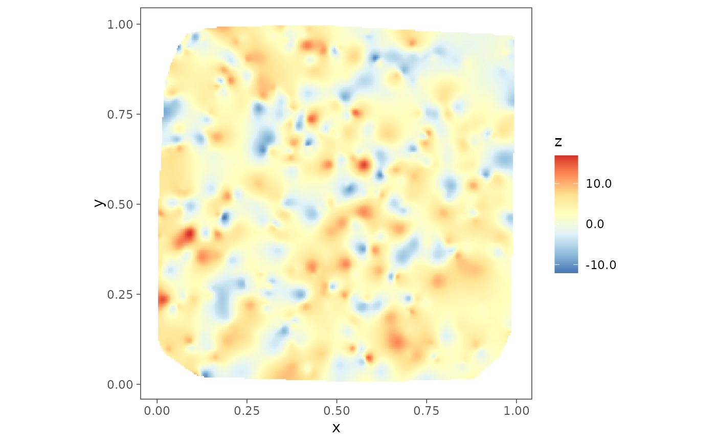
Make two side-by-side surface plots

Make two side-by-side surface plots, particularly useful towards a comparative study of two spatial surfaces.

Usage

surfaceplot2(
  tab,
  coords_name,
  var1_name,
  var2_name,
  h = 8,
  col.pal,
  mark_points = FALSE,
  titles = c(var1_name, var2_name)
)

Arguments

tab

a data-frame containing spatial co-ordinates and the variables to plot

coords_name

name of the two columns that contains the co-ordinates of the points, also used as the axis labels

var1_name

name of the column containing the first variable to be plotted

var2_name

name of the column containing the second variable to be plotted

h

integer; (optional) controls smoothness of the spatial interpolation as appearing in the MBA::mba.surf() function. Default is 8.

col.pal

Optional; color palette, preferably divergent, use colorRampPalette function from grDevices. Default is the colorblind-friendly diverging palette 'RdBu' from ColorBrewer.

mark_points

Logical; if TRUE, the input points are marked. Default is FALSE.

titles

a character vector of length 2, the titles of the two plots. Default is the names of the two variables, c(var1_name, var2_name); use NULL for no titles.

Value

a list containing two ggplot objects, which share the colour scale (one legend serves both, e.g. with patchwork::wrap_plots(plots) + patchwork::plot_layout(guides = "collect"))

Author

Soumyakanti Pan span18@ucla.edu,
Sudipto Banerjee sudipto@ucla.edu

Examples

data(simSpatial)
plots_2 <- surfaceplot2(simSpatial, coords_name = c("s1", "s2"),
                        var1_name = "z_true", var2_name = "y_gauss",
                        titles = c("True spatial effect", "Gaussian response"))
plots_2
#> [[1]]

#> 
#> [[2]]

#>